9 Martingales & friends in continuous time

9.1 Why?

Now we’ve had an introduction to stochastic processes in continuous time in the previous chapter, it is time to see what martingales look like in this world. Much of what we’re discussing in this chapter is, at least conceptually/intuitively, a natural analogue of martingales & friends in discrete time as we explored in Chapter 5–Chapter 7. However, as we already saw in Chapter 8, continuous time is at times, ehm, extra fascinating!

9.2 Filtrations

Let’s return to the core theme of this course: martingales! The definitions needed in the continuous time setting look like the natural analogues/extensions of those already discussed in discrete time (cf. Section 5.2 & Section 5.3), and the Brownian motion and Poisson process introduced in the previous Chapter 8 already provide us with numerous examples of martingales as we will see. We won’t keep repeating the qualifier “in continuous time” below, just keep in mind that everything we do in this chapter (unless explicitly mentioned otherwise) is in continuous time.

On a probability space $(\Omega,\mathcal{F},\P)$, a filtration is a collection $(\mathcal{F}_t)_{t \geq 0}$ of $\sigma$-algebras so that

$\mathcal{F}_t \subseteq \mathcal{F}$ for all $t \geq 0$,
for any $0\leq t \leq s$, $\mathcal{F}_t \subseteq \mathcal{F}_s$ (non-decreasing).

As in Section 5.2, we imagine that we walk along the time axis from time $t=0$ onwards, gathering information as we do so, and a filtration reflects that collecting of information: an event $A \in \mathcal{F}$ satisfies $A \in \mathcal{F}_t$ for some $t \geq 0$ if and only if at time $t$ we can decide whether or the not the event $A$ happens.

Adding a filtration to our probability space we obtain a filtered probability space $(\Omega,\mathcal{F},(\mathcal{F}_t)_{t \geq 0},\P)$.

A stochastic process $(X_t)_{t \geq 0}$ is said to be adapted to a filtration $(\mathcal{F}_t)_{t \geq 0}$ if it holds that $X_t$ is $\mathcal{F}_t$-measurable for all $t \geq 0$.

Given a stochastic process, its natural filtration is the filtration $(\mathcal{F}_t)_{t \geq 0}$ defined by \[\mathcal{F}_t=\sigma(X_s \, | \, s \in [0,t]) \quad \text{for all } t \geq 0\] i.e. for any $t \geq 0$, $\mathcal{F}_t$ is the smallest $\sigma$-algebra with respect to which all the random variables $X_s$ for $s \in [0,t]$ are measurable (analogue to Lemma 5.1).

Note that a process $(X_t)_{t \geq 0}$ is trivially adapted to its natural filtration $(\mathcal{F}_t)_{t \geq 0}$, and if $(\mathcal{G}_t)_{t \geq 0}$ is another filtration to which the process is adapted then necessarily $\mathcal{F}_t \subseteq \mathcal{G}_t$ for all $t \geq 0$.

Remark 9.1. As mentioned previously already, the step from discrete to continuous time also comes with some prickly technical challenges. One of these is related to filtrations. Recall that in the chapters on discrete time processes, we only ever used natural filtrations of processes — that was sufficient to discuss everything we needed, including first hitting times of Borel sets as stopping times etc.

Sadly the natural filtration of a continuous time process typically offers us no such joy. There is a standard process to make the natural filtration larger (i.e. add extra sets/events to each $\sigma$-algebra it contains) so that the resulting filtration is better behaved, typically called the usual augmentation of the natural filtration, and a filtration with the desired properties (e.g. after such an enlargement) is said to satisfy the usual conditions (I know, that’s hardly a very descriptive term — I guess that because it’s such a standard procedure in the advanced study of stochastic processes it’s common enough that it doesn’t deserve a fancier name!).

It is beyond the scope of this course (unfortunately) to say a lot more about this and so you shouldn’t worry about it for exam purposes etc. — if you’re interested in learning more, then have a look at Section 1.4 in Revuz and Yor (1993) e.g.

9.3 Martingales

On to martingales in continous time then! The definition is a straight translation from the one in discrete time (cf. Definition 5.2):

Definition 9.1 On some filtered probablity space $(\Omega,\mathcal{F},(\mathcal{F}_t)_{t \geq 0},\P)$ (cf. Section 9.2), a stochastic process $(X_t)_{t \geq 0}$ is called a martingale if it satisfies the following three conditions:

$(X_t)_{t \geq 0}$ is adapted to $(\mathcal{F}_t)_{t \geq 0}$ (cf. Section 9.2),
$(X_t)_{t \geq 0}$ is integrable — meaning that each random variable $X_t$ is integrable i.e. $\E[\lvert X_t \rvert]<\infty$ for all $t \geq 0$,
the martingale property holds: \[\E[X_t \, | \, \mathcal{F}_s]=X_s \quad \text{for all $0 \leq s < t$} \tag{9.1}\]

Further, we say that $(X_t)_{t \geq 0}$ is a submartingale resp. supermartingale if it satisfies conditions i and ii above, plus in addition the submartingale property \[\E[X_t \, | \, \mathcal{F}_s] \geq X_s \quad \text{for all $0 \leq s < t$} \tag{9.2}\] resp. the supermartingale property \[\E[X_t \, | \, \mathcal{F}_s] \leq X_s \quad \text{for all $0 \leq s < t$}. \tag{9.3}\]

Some notes:

As in discrete time, we see that a process is a martingale if and only if it is both a sub- and supermartingale.
As in discrete time, the (sub/super)martingale property uses the concept of conditional expectations — recall that we discussed these extensively in Chapter 4 and in particular the list of very useful properties we saw in Section 4.6. Further, as previously, recall that conditional expectations are defined up to almost sure equivalence only and hence the (sub/super)martingale property can only be true almost surely only.
Still as in discrete time, observe that the filtration chosen plays a crucial role in the above — if we are working on a probability space on which we have defined more than one filtration then we will/should clarify which one we are using by saying “is a (sub/super)martingale with respect to [a filtration]”.
Using the same argument as in Exercise 5.3, we may equivalently formulate the martingale property as \[\E[X_t-X_s \, | \, \mathcal{F}_s]=0 \quad \text{for all $0 \leq s < t$} \tag{9.4}\] (analogue for the sub- and supermartingale property).

The interpretations of these properties directly carry over from discrete time — maybe you want to have another quick skim through Section 5.3 to remind yourself. In particular, fixing any $0 \leq s \leq t$, taking expectations on both sides of Equation 9.1, Equation 9.2 and Equation 9.3 and using Theorem 4.2 i yields resp. \[\E[X_t]=\E[X_s], \quad \E[X_t] \geq \E[X_s], \quad \E[X_t] \leq \E[X_s] \tag{9.5}\] showing that on average, martingales resp. submartingales resp. supermartingales tend to stay constant, resp. increase, resp. decrease.

Nothing like some nice examples. Recall Brownian motion and Poisson processes as discussed in Chapter 8. Note for yourself how the independent, stationary increments property of both processes is well used in the below!

Example 9.1 Let $(B_t)_{t \geq 0}$ be a Brownian motion on a filtered probablity space $(\Omega,\mathcal{F},(\mathcal{F}_t)_{t \geq 0},\P)$, where the $(\mathcal{F}_t)_{t \geq 0}$ is the natural filtration of $(B_t)_{t \geq 0}$ (cf. Section 9.2). Then the following processes are all martingales:

$(B_t)_{t \geq 0}$ itself,
the process $(X_t)_{t \geq 0}$ given by $X_t=B_t^2-t$ for all $t \geq 0$,
the process $(X_t)_{t \geq 0}$ given by \[X_t = e^{\sigma B_t-\sigma^2 t/2} \quad \text{for all } t \geq 0,\] where $\sigma>0$ is a parameter.

Starting with $(B_t)_{t \geq 0}$ itself, we’ll check the three conditions from Definition 9.1:

Adapted: that’s obvious since we’re using the natural filtration of $(B_t)_{t \geq 0}$.
Integrable: fix any $t > 0$ (recall that $B_0=0$, cf. Definition 8.2 i, so that’s obvious). We could use that the distribution of $\lvert B_t \rvert$ is well known and that we have an expression for its expectation (as used in the proof of Proposition 8.1), but a more general approach that doesn’t rely on that specific fact is to observe that for any $x \in \R$ we have that $\lvert x \rvert \leq 1+x^2$, so that we can derive \[\E[\lvert B_t \rvert] \leq \E[1+B_t^2] \leq 1+\E[B_t^2]=1+t<\infty,\] where we used that $B_t \sim \mathcal{N}(0,t)$ (cf. the final bullet point in Definition 8.2) and hence \[t=\var(B_t)=\E[B_t^2]-\big( \E[B_t] \big)^2=\E[B_t^2]. \tag{9.6}\]
Martingale property: fix any $0 \leq s < t$. Note that with the natural filtration in the picture, Definition 8.2 iii can now be read as follows: the increment $B_t-B_s$ is independent of $\mathcal{F}_s=\sigma(B_u \, | \, u \in [0,s])$, and hence using Theorem 4.2 vi we get that \[\E[B_t-B_s \, | \, \mathcal{F}_s]=\E[B_t-B_s]=\E[B_t]-\E[B_s]=0,\] the final step using that $B_t$ and $B_s$ both have expectation $0$ (cf. the final bullet point in Definition 8.2), so indeed Equation 9.4 holds.

Just for the full picture: of course you could also use the “original” martingale property i.e. Equation 9.1. For that one, we still want to make use of the nice properties we know about increments of Brownian motion by “bringing in” an increment: \[\E[B_t \, | \, \mathcal{F}_s]=\E[B_t-B_s+B_s \, | \, \mathcal{F}_s]=\E[B_t-B_s \, | \, \mathcal{F}_s]+B_s,\] where we used linearity of conditional expectations, as well as that $B_s$ is obviously $\mathcal{F}_s=\sigma(B_u \, | \, u \in [0,s])$-measurable together with Theorem 4.2 ii. Then we can use the same argument as above to show that $\E[B_t-B_s \, | \, \mathcal{F}_s]=0$ and hence we’re done.

Next let’s do the process defined in 2, $(X_t)_{t \geq 0}$ given by $X_t=B_t^2-t$ for all $t \geq 0$ We check the same three properties:

Adapted: $B_t^2$, being a (smooth) function of $B_t$ is $\mathcal{F}_t=\sigma(B_s \, | \, s \in [0,t])$-measurable and that remains the case if we subtract the constant $t$.
Integrable: for any $t \geq 0$, the triangle inequality yields $\lvert X_t \rvert \leq B_t^2 + t$ and hence \[\E[\lvert X_t \rvert] \leq \E[B_t^2]+t \leq 2t<\infty,\] where we also used Equation 9.6 again.
Martingale property: fix any $0 \leq s < t$. The trick is again to find a way to bring an increment into play — any way is fine of course, here is one possibility: \[\begin{align*} \E[X_t \, | \, \mathcal{F}_s] &= \E[B_t^2-t \, | \, \mathcal{F}_s] \\ &= \E[(B_t-B_s+B_s)^2-t \, | \, \mathcal{F}_s] \\ &= \E[(B_t-B_s)^2+2B_s(B_t-B_s)+B_s^2-t \, | \, \mathcal{F}_s] \\ &= \E[(B_t-B_s)^2 \, | \, \mathcal{F}_s] + 2 \E[B_s(B_t-B_s) \, | \, \mathcal{F}_s] + \E[B_s^2 \, | \, \mathcal{F}_s]-t \\ &= \E[(B_t-B_s)^2]+2B_s\E[B_t-B_s]+B_s^2-t \\ &= t-s+B_s^2-t \\ &= X_s. \end{align*} \] The fourth line first uses linearity of conditional expectations. The fifth line works out the conditional expectations: the first term uses that $(B_t-B_s)^2$ is a function of the increment $B_t-B_s$ and therefore independent of $\mathcal{F}_s$ (cf. Definition 8.2 iii) so that we can use Theorem 4.2 vi; the second term uses first that $B_s$ is $\mathcal{F}_s$-measurable together with Theorem 4.2 v to take it out, and then the same argument as for the first term; finally the third term uses that $B_s^2$, being a function of $B_s$, is $\mathcal{F}_s$-measurable and hence Theorem 4.2 ii applies. The sixth line uses that $B_t-B_s \sim \mathcal{N}(0,t-s)$ (cf. Definition 8.2 iv) as well as Equation 9.6 again.

Note: there are alternative valid ways to “bring in an increment” above, however please do have the following crucial subtlety sharp for yourself: $B_t-B_s$ is independent of $\mathcal{F}_s$ and hence so is any function of $B_t-B_s$, like $(B_t-B_s)^2$ since we can write it as $g(B_t-B_s)$ for $g(x)=x^2$; but (e.g.) $B_t^2-B_s^2$ is not a function of $B_t-B_s$ so that same argument is invalid for this expression!

The third one we leave for you to do in Exercise 9.1!

Let’s also look at Poisson processes, the other important example of continuous time processes we discussed in Chapter 8:

Example 9.2 Now consider a Poisson process $(N_t)_{t \geq 0}$ with intensity $\lambda>0$ (cf. Definition 8.4) on a filtered probablity space $(\Omega,\mathcal{F},(\mathcal{F}_t)_{t \geq 0},\P)$, where the $(\mathcal{F}_t)_{t \geq 0}$ is the natural filtration of $(N_t)_{t \geq 0}$ (cf. Section 9.2).

Firstly, note that $(N_t)_{t \geq 0}$ itself is not a martingale. Indeed, a quick way to see this is to observe that since for any $t>0$, $N_t \sim \text{Poisson}(\lambda t)$ (cf. Definition 8.4 iv), we have that $\E[N_t]=\lambda t$ so it fails to have a constant expectation as would be required (cf. Equation 9.5).

On second thought, this is no surprise of course: we have seen that the paths of a Poisson process are non-decreasing (cf. Section 8.4.1), so for any $0 \leq t_1 \leq t_2$ and $\omega \in \Omega$ we have that $N_{t_2}(\omega) \geq N_{t_1}(\omega)$, i.e. as random variables we have that $N_{t_2} \geq N_{t_1}$ (pointwise). With positive probability (namely if we have at least one occurence in the time interval $(t_1,t_2]$) it holds that $N_{t_2} > N_{t_1}$. So from this argument it also follows that $\E[N_{t_2}]>\E[N_{t_1}]$, as the explicit computation in the previous paragraph already showed.

On the other hand, Poisson processes do share that nice stationary, independent increment property with Brownian motion, which as we saw in Example 9.1 goes a long way to guaranteeing martingale like behaviour. Indeed, all we really need to do is “compensate” $(N_t)_{t \geq 0}$ by subtracting its expectation to arrive at a martingale: the process $(X_t)_{t \geq 0}$ given by \[X_t = N_t-\E[N_t]=N_t-\lambda t \quad \text{for all } t \geq 0\] is a martingale. Indeed, you can easily check that it’s adapted and integrable yourself, and to check the martingale property (cf. Definition 9.1), note that for any $0 \leq s<t$ we can reason very similarly as for Brownian motion in Example 9.1 by “bringing in an increment”: \[\begin{align*} \E[X_t \, | \, \mathcal{F}_s] &= \E[N_t-\lambda t \, | \, \mathcal{F}_s] \\ &= \E[N_t-N_s+N_s-\lambda t \, | \, \mathcal{F}_s] \\ &= \E[N_t-N_s \, | \, \mathcal{F}_s] + \E[N_s \, | \, \mathcal{F}_s] - \lambda t \\ &= \E[N_t-N_s] + N_s - \lambda t \\ &= \lambda (t-s) + N_s - \lambda t \\ &= X_s, \end{align*} \] where the fourth line uses that the increment $N_t-N_s$ is independent of $\mathcal{F}_s=\sigma(N_u \, | \, u \in [0,s])$ (cf. Definition 8.4 iii) with Theorem 4.2 vi and that $N_s$ is $\mathcal{F}_s$-measurable with Theorem 4.2 ii, and the fifth line uses that $N_t-N_s \sim \text{Poisson}(\lambda (t-s))$ (cf. Definition 8.4 iv).

Exercises

You can now do Exercise 9.1–Exercise 9.3.

9.4 Stopping times

We can also naturally extend the idea of a stopping time from discrete to continuous time. Recall the discrete time case from Section 6.2. In continuous time we have the following analogue def:

Definition 9.2 On a filtered probablity space $(\Omega,\mathcal{F},(\mathcal{F}_t)_{t \geq 0},\P)$, a stopping time (with respect to $(\mathcal{F}_t)_{t \geq 0}$) is a mapping $\tau: \Omega \to [0,\infty]$ with the property that \[\{ \tau \leq t\} \in \mathcal{F}_t \quad \text{for all } t \geq 0. \tag{9.7}\]

Recall that we use $[0,\infty]:=[0,\infty) \cup \{\infty\}$, so we explicitly allow for the possibility that $\tau$ (also) takes the value $\infty$. By the same arguments used in Section 6.2, any such $\tau$ is automatically $\mathcal{F}$-measurable and hence a (non-negative) random variable.

Comparing & contrasting this def with the one in discrete time, cf. Definition 6.1, note that it does not make sense to (rigorously) talk about \[\{ \tau = t\} \in \mathcal{F}_t \quad \text{for all } t \geq 0\] as equivalent for Equation 9.7 — the problem is that, contrary to discrete time, there are uncountably many $t$ for which we’d have to consider the event $\{ \tau = t\}$ etc.

The interpretation of a stopping time $\tau$ in continuous time is the same as in discrete time: we think about it as a random point on the time axis $[0,\infty)$, and the condition Equation 9.7 can be read as follows: if you imagine walking along the time axis from time $t=0$ onwards, then the decision to pick a time point to be your value for $\tau$ may only depend on what you have so far observed, up until that time point, and not on anything that may or may not happen after that time point.

Your typical example of a stopping time $\tau$ arises in conjunction with an adapted process $(X_t)_{t \geq 0}$, by looking at $\tau(\omega)$ defined as the first time that the path $t \mapsto X_t(\omega)$ does [thing], where [thing] must be something so that at every $t \geq 0$, you can decide whether or not [thing] happens based on the part of the path you have so far observed i.e. $s \mapsto X_s(\omega)$ for $s \in [0,t]$ (if using the natural filtration of $(X_t)_{t \geq 0}$).

Within this class of examples, first hitting/entry times are particularly prominent — it is a direct translation from the same concept in discrete time (cf. Example 6.1) but comes with some additional technical challenges in continuous time! In general, for a Borel set $C \subseteq \R$, we look at the first time that an adapated process $(X_t)_{t \geq 0}$ hits/enters $C$ i.e. \[\tau(\omega) := \inf \{ t \geq 0 \, | \, X_t(\omega) \in C \} \quad \text{for } \omega \in \Omega,\] with the understanding that $\inf \emptyset:=\infty$. Note that this kicks in if $t \mapsto X_t(\omega)$ never hits/enters $C$ i.e. $X_t(\omega) \not\in C$ for all $t \geq 0$, since then \[\{ t \geq 0 \, | \, X_t(\omega) \in C \}=\emptyset.\] Recall that “inf” is short for “infimum”, see e.g. Wiki if you’d like a reminder.

Recall that in discrete time, any first hitting/entry time is a stopping time (cf. Example 6.1) but no such convenience in continuous time unfortunately! :(.

Example 9.3 Suppose that $(X_t)_{t \geq 0}$ is a continuous process on a filtered probablity space $(\Omega,\mathcal{F},(\mathcal{F}_t)_{t \geq 0},\P)$, with $X_0=0$, and let $(\mathcal{F}_t)_{t \geq 0}$ be the natural filtration of $(X_t)_{t \geq 0}$ i.e. $\mathcal{F}_t=\sigma(X_s \, | \, s \in [0,t])$ for all $t \geq 0$.

Consider for instance the first entry time of $(a,\infty)$ for some $a>0$ fixed: \[\tau = \inf \{ t \geq 0 \, | \, X_t >a \}=\inf \{ t \geq 0 \, | \, X_t \in (a,\infty) \}.\] This is (generally) not a stopping time!

Here is why — intuitively at least. Consider a path $t \mapsto X_t(\omega)$ so that $X_t(\omega)<a$ for all $t \in [0,1)$ and $X_1(\omega)=a$ (the choice for the timepoint $1$ is arbitary, just as example). Consider the following two (non-exhaustive) scenarios:

for some $h>1$, $X_t(\omega)<a$ for all $t \in (1,h]$. So after reaching the level $a$ in $t=1$, the path decreases for a little while (at least). Then we have that $X_t(\omega)<a$ for all $t \in [0,h]$ and hence $\tau(\omega) \geq h>1$.
for some $h>1$, $X_t(\omega)>a$ for all $t \in (1,h]$. So after reaching the level $a$ in $t=1$, the path increases for a little while (at least). Then any $t \in [0,1]$ is not in the set \[\{ t \geq 0 \, | \, X_t \in (a,\infty) \}\] but any $t \in (1,h]$ is in this set. Then the infimum of this set is the same as the infimum of $(1,h]$ which equals $1$, hence $\tau(\omega)=1$.

Note that in scenario 1 we have that $\tau(\omega)>1$ while in scenario 2 we have that $\tau(\omega)=1$. So standing at time $t=1$ and having observed the path to this moment, we can’t decide whether we are stopping now i.e. $\tau(\omega)=1$ or whether we should wait longer i.e. $\tau(\omega)>1$… More mathematically, using the information available in $\mathcal{F}_1=\sigma(X_s \, | \, s \in [0,1])$, we cannot decide whether we are dealing with an $\omega$ from $\{ \tau \leq 1 \}$ or not, i.e. $\{ \tau \leq 1 \} \not\in \mathcal{F}_1$ so that Equation 9.7 fails to hold and hence $\tau$ fails to be a stopping time.

Ok, so how do we pick up and glue back together the pieces?? Basically in two parts. First, as you may have noted, fundamentally the problem in Example 9.3 is caused by the fact that we are looking at the first entry time of an open Borel set, so that it is possible to hoover exactly at the boundary of the set to enter it immediately after or rather move away from it. This is not possible with the first entry time of closed Borel sets. Since a continuous process can only enter a closed Borel set by hitting its boundary — e.g., a continuous process starting from level $0$ can only enter the interval $[2,4]$ by hitting the level $2$, as opposed to a cadlag process whose paths have jumps, like a Poisson process, which can enter a Borel set by jumping somewhere inside of it — it is for these purposes enough to look at first hitting times of a level:

Lemma 9.1 On a filtered probablity space $(\Omega,\mathcal{F},(\mathcal{F}_t)_{t \geq 0},\P)$, let $(X_t)_{t \geq 0}$ be a continuous process and $(\mathcal{F}_t)_{t \geq 0}$ its natural filtration. Fix any $x \in \R$. Then \[\tau = \inf \{ t \geq 0 \, | \, X_t =x \}\] is a stopping time.

Proof. Clearly we’ll need to prove that Equation 9.7 holds. First to get a special case out of the way, note that \[\{\tau \leq 0 \}=\{\tau=0\}=\{X_0=x\} \in \mathcal{F}_0,\] since $X_0$ is $\mathcal{F}_0=\sigma(X_0)$-measurable.

Now fix some $T > 0$ and consider a path $t \mapsto X_t(\omega)$. Our general strategy is to try and mimic the argument we used in discrete time (cf. Equation 6.4): express $\tau(\omega) \leq T$ in terms of the path of $t \mapsto X_t(\omega)$ on the time interval $[0,T]$ (step 1), and do that in such a way that we can use the fact that $(X_t)_{t \geq 0}$ is adapted to conclude that Equation 9.7 holds (step 2). All a bit more fiddly than in discrete time though!

Step 1. Note that by continuity and the extreme value theorem & intermediate value theorem, the set of values visited by $t \mapsto X_t(\omega)$ for $t \in [0,T]$ i.e. its range is an interval $[a,b] \subseteq \R$ (nothing magical here, just saying that a continuous function on $[0,T]$ attains both its minimal value $a$, maximal value $b$, as well as any value in between these). We claim that \[\tau(\omega) \leq T \iff \text{there exists a } t_0 \in [0,T] \text{ so that } X_{t_0}(\omega)=x \iff x \in [a,b]. \tag{9.8}\] For a proof, note that the second equivalence is trivial by def of the range $[a,b]$ so we only need to deal with the first equivalence. To see this:

if $x \not\in [a,b]$, since $X_t(\omega) \in [a,b]$ for all $t \in [0,T]$ and since there is a positive distance between $x$ and $[a,b]$, by continuity of the path there exists $h>0$ so that $X_t(\omega) \not=x$ for all $t \in [0,T+h]$, implying that \[\{ t \geq 0 \, | \, X_t(\omega) =x \} \subseteq (T+h,\infty)\] and hence $\tau(\omega) \geq \inf \, (T+h,\infty) = T+h$, i.e. $\tau(\omega) \leq T$ does not hold.
if $x \in [a,b]$ so that there exists a $t_0 \in [0,T]$ so that $X_{t_0}(\omega)=x$, then \[t_0 \in \{ t \geq 0 \, | \, X_t(\omega) =x \}\] and hence $\tau(\omega) \leq t_0 \leq T$.

Step 2. Next, it is tempting to use Equation 9.8 to write the event $\{\tau \leq T\}$ as the union over $t \in [0,T]$ of events $\{ X_t=x \}$, but this is useless: as already discussed in Section 8.2, this is a union consisting of uncountably many events and hence we cannot argue that it is contained in $\mathcal{F}_T$. Rather we need to go via the rational numbers again. This is in this situation a bit tricky to formulate though! We claim that each statement in Equation 9.8 is also equivalent to the following statement: \[\text{for any } n=1,2,\ldots \text{ there exists a } q_n \in \Q \cap [0,T] \text{ so that } \lvert X_{q_n}(\omega)-x \rvert<\frac{1}{n}. \tag{9.9}\] For a proof of this claim:

Suppose that all statements in Equation 9.8 hold. We use in particular the middle one. Fix some $n=1,2,\ldots$. By continuity of the path, there exists a $\delta>0$ so that for all $t \in (t_0-\delta,t_0+\delta)$ we have that $\lvert X_t(\omega)-x \rvert<1/n$. Because $\Q$ is dense in $\R$ (cf. Proposition 1.2 iv), this interval $t \in (t_0-\delta,t_0+\delta)$ also contains an element from $\Q \cap [0,T]$ wich we can take to be our $q_n$.
Suppose that Equation 9.9 holds. Note that Equation 9.9 defines a sequence of numbers in $[0,T]$, $q_n$ for $n=1,2,\ldots$, so that $X_{q_n}(\omega) \to x$ as $n \to \infty$. By def of the range $[a,b]$, it holds that $X_{q_n}(\omega) \in [a,b]$ for all $n=1,2,\ldots$, and since $[a,b]$ is closed also their limit $x$ is an element of $[a,b]$ (recall that this is a defining property of closed sets in general, see e.g. Wiki). So the right hand statement in Equation 9.8 holds.

Now we’re finally there: combining Equation 9.8 and Equation 9.9, we see for any $\omega \in \Omega$ that $\tau(\omega) \leq T$ holds if and only if Equation 9.9 holds. In terms of events this becomes: \[\{ \tau \leq T\} = \bigcap_{n=1,2,\ldots} \bigcup_{q \in \Q \cap [0,T]} \left\{ \lvert X_{q}(\omega)-x \rvert<\frac{1}{n} \right\}.\] For any $n=1,2,\ldots$ and $q \in \Q \cap [0,T]$ fixed we have that \[\left\{ \lvert X_{q}(\omega)-x \rvert<\frac{1}{n} \right\} \in \mathcal{F}_q \subseteq \mathcal{F}_T,\] since $X_q$ is $\mathcal{F}_q$-measurable and a filtration is non-decreasing (cf. Section 9.2). By the usual $\sigma$-algebra properties, for any $n=1,2,\ldots$ fixed the union over $q \in \Q \cap [0,T]$ of these events is also in $\mathcal{F}_T$ (cf. Definition 1.1 iii) and then so is the intersection over $n=1,2,\ldots$ of these unions (cf. Proposition 1.1 i).

The second part of our road to salvation is the observation that in Example 9.3, if only we had a tiny bit more information at time $t=1$, namely what happens “immediately after” time $t=1$, we would have had no problem. As already alluded to in Remark 9.1, there is a standard process (the “usual augmentation”) to enlarge the natural filtration somewhat to one that satisfies the “usual conditions”, and under this enlarged filtration there are no more problems — not only for continuous processes but neither for cadlag processes, the first hitting/entry time of any Borel set is then guaranteed to be a stopping time. This general result is commonly known as the Début theorem, see e.g. Theorem 4.15 in Revuz and Yor (1993) if you’re interested.

As a little aside: you may wonder why we at all bother with natural filtrations then, why not use this enlarged filtration from the start of this chapter and avoid much of this hassle altogether? Well we could do that, but then we just end up moving the hassle around: for the examples of martingales that we have seen, being able to use the natural filtration made the arguments relatively straightforward. If we’d have to use a larger filtration these arguments would become less obvious — the results are still true i.e. the martingales we have seen are also martingales with respect to the filtration obtained by “usual augmentation” of the natural filtration involved, but the proof would be considerably harder.

9.4.1 Stopped processes

As in discrete time (cf. Section 6.3), when on some filtered probability space $(\Omega,\mathcal{F},(\mathcal{F}_t)_{t \geq 0},\P)$ we have a stopping time $\tau$ and an adapted process $(X_t)_{t \geq 0}$, we are often interested in the stopped process $(X^\tau_t)_{t \geq 0}=(X_{t \wedge \tau})_{t \geq 0}$¹: we keep the process $(X_t)_{t \geq 0}$ unchanged up until time $\tau$, but from time $\tau$ onwards we stay fixed at the level $X_\tau$. Recall that “$t \wedge s$” is just shorthand notation for “$\min\{t,s\}$”.

¹ Recall, as in discrete time, that the notation “${X}^{\tau}$” here does not indicate a power but is rather a label only indicating that we’re dealing with a stopped process

In terms of random variables that means, for any time $t \geq 0$ fixed, that the random variable $X^\tau_t=X_{t \wedge \tau}$ is equal to $X_t$ if $t<\tau$ (i.e. on the event that we haven’t stopped yet at time $t$) and equal to $X_\tau$ if $t \geq \tau$ (i.e. on the complementary event that we have stopped already). In formulas: \[X^\tau_t=X_{t \wedge \tau}=\mathbf{1}_{\{ t<\tau \}} X_t + \mathbf{1}_{\{ t \geq \tau \}} X_\tau=\begin{cases} X_t & \text{if } t<\tau \\ X_\tau & \text{if } t \geq \tau \end{cases} \quad \text{for all } t \geq 0. \tag{9.10}\] Of course we can also take the path perspective: for any $\omega \in \Omega$, the path of the stopped process $t \mapsto X^\tau_t(\omega)=X_{t \wedge \tau(\omega)}(\omega)$ follows the path $t \mapsto X_t(\omega)$ up until time $\tau(\omega)$, but after this time the path of the stopped process stays constantly fixed at the level it was at at time $\tau(\omega)$, namely $X_{\tau(\omega)}(\omega)$.

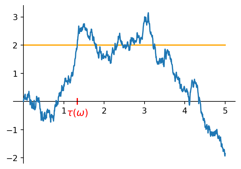
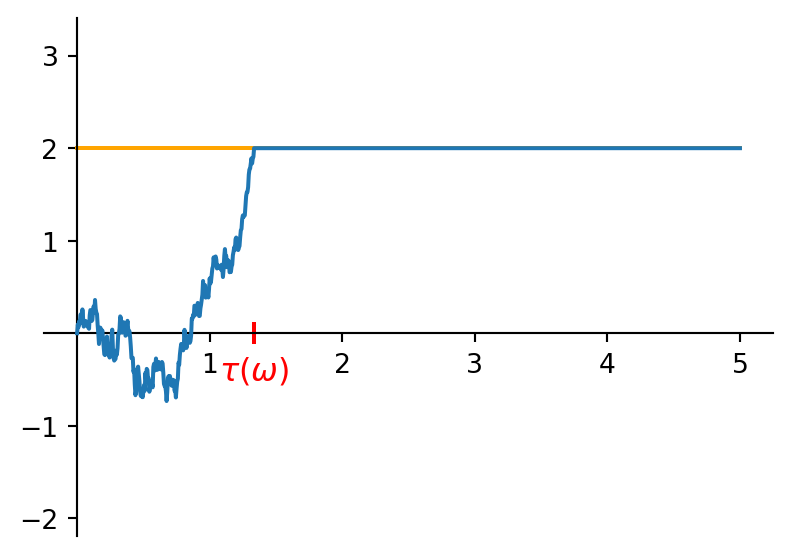
Example 9.4 Take for instance a Brownian motion $(B_t)_{t \geq 0}$ (cf. Section 8.3) on a filtered probability space $(\Omega,\mathcal{F},(\mathcal{F}_t)_{t \geq 0},\P)$, where $(\mathcal{F}_t)_{t \geq 0}$ is the natural filtration of $(B_t)_{t \geq 0}$. And let’s take the first hitting time of the level $a \in \R$ i.e. \[\tau=\inf \{ t \geq 0 \, | \, B_t=a \}. \tag{9.11}\] Recall from Lemma 9.1 that this is indeed a stopping time. Figure 9.1 shows a visual of a path and the corresponding path of the stopped process for the case $a=2$. Having a quick look back at Corollary 8.1, since with probability $1$ a path of Brownian motion hits any level $a \in \R$ (even infinitely often), we have that $\tau<\infty$ a.s.

Further observe that for any $\omega \in \Omega$, if $\tau(\omega)<\infty$ then the path hits the level $a$ at time $\tau(\omega)$ i.e. we have that $X_{\tau(\omega)}(\omega)=a$. As is the case for most processes, we mentioned already that $\tau<\infty$ a.s. but we can’t guarantee that this is true pointwise. For any $\omega \in \Omega$ with $\tau(\omega)=\infty$ we have to leave $X_{\tau(\omega)}(\omega)$ undefined, as we also did in the discrete time case (recall from Section 7.3.1 e.g.). However, as we know well by now, as long as this happens with probability $0$ only it doesn’t matter a lot since probability $0$ events do not affect the distribution for instance (recall from Exercise 2.9).

It is nice, I think, to compare and contrast a bit with a process whose paths are not continuous i.e. have jumps/discontinuities, like a Poisson process $(N_t)_{t \geq 0}$ (cf. Section 8.4) on a filtered probability space $(\Omega,\mathcal{F},(\mathcal{F}_t)_{t \geq 0},\P)$ — where we assume that the filtration $(\mathcal{F}_t)_{t \geq 0}$ is the natural filtration enlarged to satisfy the “usual conditions” to ensure that any first hitting/entry time is a stopping time (cf. Remark 9.1). If we consider a first hitting time \[\tau=\inf \{ t \geq 0 \, | \, N_t=a \},\] then it makes a big difference how we choose the level $a$! E.g. if we take some $a \geq 0$ which is not an integer, then it is essentially impossible for a path to hit $a$ since typical paths only visit the non-negative integers (recall e.g. the pic from Figure 8.2) — e.g. if you take some $a \in (2,3)$ then a path with $N_0(\omega)=0$ will at some point jump from level $2$ to level $3$ i.e. cross $a$ without actually hitting it and will carry on increasing over time, so that $\{ t \geq 0 \, | \, N_t(\omega)=a \}=\emptyset$ and hence $\tau(\omega)=\infty$!

Aside: we say “essentially impossible” above because the definition of a Poisson process specifies that $N_0=0$ is true almost surely only (cf. Definition 8.4), a different value for $N_0$ could potentially lead to hitting $a$ but this happens with probability $0$ only.

Therefore, when dealing with a process with jumps, we normally prefer to use first entry times of an interval (for instance) rather than the first hitting time of a level, e.g. \[\tau=\inf \{ t \geq 0 \, | \, N_t \geq a \}. \tag{9.12}\] Keep in mind that the presence of jumps generally also complicates the level the process is stopped at. For instance, if we take some $a \in (2,3)$ and consider Equation 9.12 then we will have, provided $\tau(\omega)<\infty$ that $N_{\tau(\omega)}(\omega)=3>a$. And for we can still use the special structure that a Poisson process has — if $(N_t)_{t \geq 0}$ would rather be some process that can have have jumps of any size then all we can in general really is that $N_{\tau(\omega)}(\omega) \geq a$!

(a) In blue a path of a Brownian motion $t \mapsto B_t(\omega)$ for $t \in [0,5]$. Note that the level $2$ (in orange) is hit at multiple time points, and each of these time points goes into the set $\{ t \geq 0 \, | \, B_t(\omega)=2 \}$. The infimum i.e. (roughly speaking) smallest of them is $\tau(\omega) \approx 1.33$

Finally on this topic, recall that in discrete time, it was not very hard to see that a stopped martingale is still a martingale, cf. Proposition 6.1. The result is still true in continuous time:

Proposition 9.1 On some filtered probability space $(\Omega,\mathcal{F},(\mathcal{F}_t)_{t \geq 0},\P)$, suppose that $(X_t)_{t \geq 0}$ is a cadlag (sub/super)martingale and $\tau$ a stopping time. Then the stopped process $(X^\tau_t)_{t \geq 0}=(X_{t \wedge \tau})_{t \geq 0}$ (cf. Equation 9.10) is also a cadlag (sub/super)martingale.

Contrary to discrete time, this is quite hard to prove though! We’ll discuss some aspects of this in Exercise 9.5.

Exercises

You can now do Exercise 9.4–Exercise 9.5.

9.5 Dooooob!

Now we have set the scene and introduced martingales, stopping times and stopped processes in continuous time, a very natural question to ask is the following. In Chapter 5 & Chapter 6 we saw and discussed a number of fundamental results, (mostly) by the heroic Doob, for discrete time martingales. Are they still true, in some suitable analogue form, in continuous time? The answer is generally yes!

We’ll formulate and discuss them, but we won’t attempt to prove them. The general approach is to make smart use of the discrete time results, as follows. Given a continuous time cadlag martingale $(X_t)_{t \geq 0}$ on some filtered probability space $(\Omega,\mathcal{F},(\mathcal{F}_t)_{t \geq 0},\P)$, consider for some (large) integer $k$ the equidistant time grid \[\{n 2^{-k} \, | \, n \in \N\}=\{0,2^{-k},2 \cdot 2^{-k},3 \cdot 2^{-k}, \ldots\}\] and use it discretise both the process and filtration i.e. define on that same probability space $(\Omega,\mathcal{F},\P)$ the discrete time process $(Z_n)_{n=0,1,\ldots}$ given by \[Z_n = X_{n 2^{-k}} \quad \text{for all } n=0,1,\ldots\] and the discrete time filtration $(\mathcal{G}_n)_{n=0,1,\ldots}$ given by \[\mathcal{G}_n=\mathcal{F}_{n 2^{-k}} \quad \text{for all } n=0,1,\ldots.\] Then it can be shown that $(Z_n)_{n=0,1,\ldots}$ inherits the martingale property (with respect to $(\mathcal{G}_n)_{n=0,1,\ldots}$) so that discrete time results apply, and then take the limit for $k \to \infty$ to carry these over to $(X_t)_{t \geq 0}$. The cadlag property of $(X_t)_{t \geq 0}$ is an important ingredient to make this convergence work, in the spirit of Exercise 8.1. If you’re interested in more details, see e.g. Chapter II in Revuz and Yor (1993).

We don’t discuss a continuous time analogue of Doob’s decomposition theorem (cf. Theorem 5.1) here — it definitely exists (not in the same generality though) but is more subtle than in discrete time and needs some additional notions etc. beyond the scope of this course. If you’re interested, see e.g. Section 1.4 in Karatzas and Shreve (2000).

9.5.1 Martingale convergence theorem

Remember the martingale convergence theorem from Theorem 5.2, which we proved using the idea of counting upcrossings of intervals and being able to bound these. The analogue in continuous time is a straightforward translation of the discrete time version.

Theorem 9.1 Let $(X_t)_{t \geq 0}$ be a cadlag (sub/super)martingale on a filtered probability space $(\Omega,\mathcal{F},(\mathcal{F}_t)_{t \geq 0},\P)$ with the property that a $c>0$ exists so that $\E[\lvert X_t \rvert] \leq c$ for all $t \geq 0$. Then there exists an integrable random variable $V$ on this space so that $X_t \stackrel{\text{a.s.}}{\longrightarrow} V$ as $t \to \infty$.

9.5.2 Optional stopping theorem

Recall the optional stopping results from Section 6.4 — also in continuous time we have established in Proposition 9.1 that if $(X_t)_{t \geq 0}$ is martingale and $\tau$ a stopping time, that the stopped process $(X^\tau_t)_{t \geq 0}$ is still a martingale. By the constant expectation property (cf. Equation 9.5) this implies that \[\E[X^\tau_t]=\E[X_0] \text{ i.e. } \E[X_{t \wedge \tau}]=\E[X_0] \quad \text{for all } t \geq 0.\] It is tempting to think that, under some suitable integrability condition and provided that $\tau<\infty$ a.s. so that the random variable $X_\tau$ is well defined up to an event of probability $0$ at least, we should be able to apply the DCT (cf. Theorem 3.3) to take the limit for $t$ to $\infty$ to arrive at \[\E[X_{\tau}]=\E[X_0].\] Indeed that’s the case (in the discrete time case, we called part i below Hunt’s optional stopping theorem and part ii Doob’s optional stopping theorem):

Theorem 9.2 Let $(X_t)_{t \geq 0}$ be a cadlag martingale on a filtered probability space $(\Omega,\mathcal{F},(\mathcal{F}_t)_{t \geq 0},\P)$. Then we have the following.

If $\tau, \sigma$ are two a.s. bounded stopping times such that $\tau \geq \sigma$ a.s., then \[\E[X_\tau]=\E[X_\sigma]. \tag{9.13}\]
Further, if $\tau$ is a stopping time so that one of the following two conditions hold:
1. $\tau$ is a.s. bounded, or
2. $\tau<\infty$ a.s. and there exists an integrable random variable $Y$ so that $\lvert X_{t \wedge \tau} \rvert \leq Y$ for all $t \geq 0$ holds a.s.
then we have that \[\E[X_\tau]=\E[X_0]. \tag{9.14}\]

If $(X_t)_{t \geq 0}$ be a cadlag submartingale resp. supermartingale rather, then these results remain true provided we replace the “$=$” in Equation 9.13 & Equation 9.14 by “$\geq$” resp. “$\leq$”.

9.5.3 Maximal inequalities

Recall that the maximal inequalities (cf. Section 6.5) use the special dependency structure between the random variables making up a martingale to bound how large a martingale can get. For a cadlag process $(X_t)_{t \geq 0}$ we introduce its running supremum process $(X^*_t)_{t \geq 0}$ defined as \[X^*_t = \sup_{s \in [0,t]} \lvert X_s \rvert \in [0,\infty) \quad \text{for all } t \geq 0. \tag{9.15}\] Contrary to the discrete time case in Section 6.5, where we could safely work with the maximum in Equation 6.15 since we wanted the largest of a finite set of values, we need to work with the supremum rather now. In the special case that $(X_t)_{t \geq 0}$ is continuous we could still choose the maximum if we preferred, because each continuous path will attain its maximum on any time interval $[0,t]$ (just the extreme value theorem) but in the case of cadlag paths this is no longer necessarily the case!

Example 9.5 Consider the function $f:[0,1] \to \R$ given by \[f(x)=\begin{cases} x & \text{if } x \in [0,1/2) \\ 0 & \text{if } x \in [1/2,1]. \end{cases} \] Note that $f$ is cadlag (recall Equation 8.4 & Equation 8.5): the only point with any doubt would be $x=1/2$, but there it is right-continuous since \[\lim_{x \downarrow 1/2} f(x)=\lim_{x \downarrow 1/2} 0 = 0 \quad \text{and} \quad f(1/2)=0\] as well as an existing left limit: \[\lim_{x \uparrow 1/2} f(x)=\lim_{x \uparrow 1/2} x = 1/2.\]

Now, this function clearly does not attain its maximum: it gets arbitrarily close to the value $1/2$ but never attains it. So its maximum does not exist. Its supremum does exist and equals $1/2$ i.e. \[\sup_{x \in [0,1]} f(x)=1/2.\]

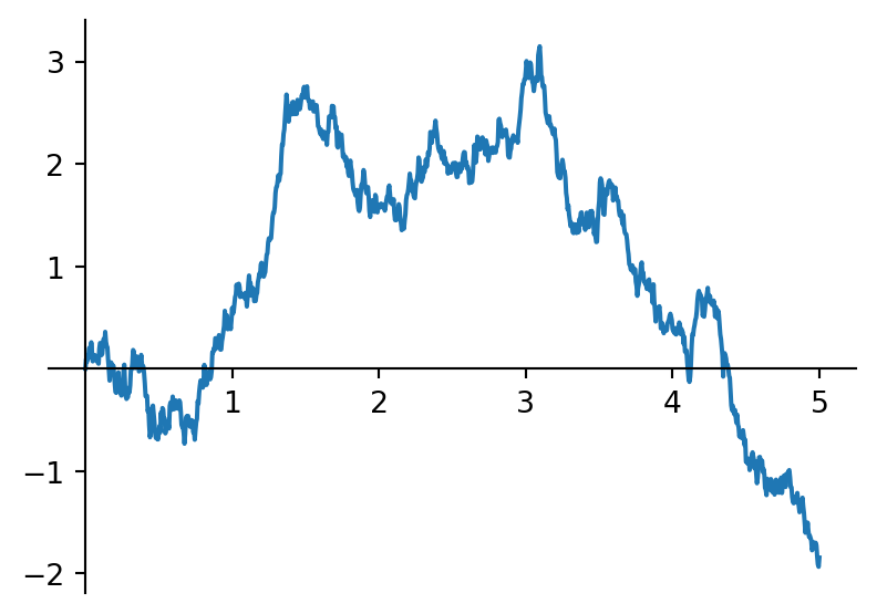
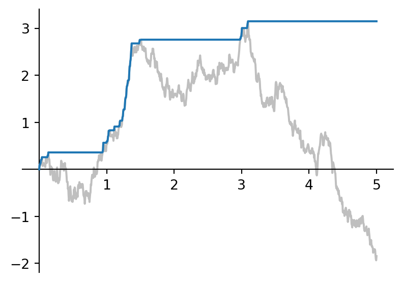
Observe that any path of the running supremum process i.e. \[t \mapsto X^*_t(\omega) = \sup_{s \in [0,t]} \lvert X_s(\omega) \rvert\] is non-decreasing (after all, if we increase $t$ then we make the time interval over which we take supremum only larger) and you can also check that it is cadlag — it experiences a jump (upwards, because non-decreasing) at a time point $t_0$ exactly if the corresponding path $t \mapsto X_t(\omega)$ has an upwards at time $t_0$ to a level higher than any level previously attained. If $(X_t)_{t \geq 0}$ is continuous then so is it running supremum process.

See Figure 9.2 for a visual illustration of the supremum process. Have a stare at it!

Further observe that due to its non-decreasing nature, we can also consider the supremum over all $t \in [0,\infty)$ as a limit i.e. the random variable $X^*_\infty$ defined as \[X^*_\infty(\omega) := \sup_{t \geq 0} \lvert X_t(\omega) \rvert = \lim_{t \to \infty} X^*_t(\omega) \in [0,\infty] \quad \text{for all } \omega \in \Omega\] (observe that it may well take the value $\infty$).

Here is what the maximal inequalities look like in continuous time:

Theorem 9.3 Let $(X_t)_{t \geq 0}$ be a cadlag process on a filtered probability space $(\Omega,\mathcal{F},(\mathcal{F}_t)_{t \geq 0},\P)$ which is one of the following:

a martingale,
a non-negative submartingale,
a non-positive supermartingale.

Let $(X^*_t)_{t \geq 0}$ be the corresponding running supremum process as introduced above. Then we have the following.

Maximal inequality: for any $\lambda>0$, \[\lambda \P(X^*_t \geq \lambda) \leq \sup_{s \in [0,t]} \E[\lvert X_s \rvert] \quad \text{for all } t \geq 0\] and \[\lambda \P(X^*_\infty \geq \lambda) \leq \sup_{t \geq 0} \E[\lvert X_t \rvert].\]
$L^p$ inequality: for any $p>1$, \[\E[(X^*_t)^p] \leq \left( \frac{p}{p-1} \right)^p \sup_{s \in [0,t]} \E[\lvert X_s \rvert^p] \quad \text{for all } t \geq 0\] and \[\E[(X^*_\infty)^p] \leq \left( \frac{p}{p-1} \right)^p \sup_{t \geq 0} \E[\lvert X_t \rvert^p].\]

(a) A path of a Brownian motion $t \mapsto X_t(\omega)$ for $t \in [0,5]$

Exercises

You can now do Exercise 9.6–Exercise 9.9.

9.6 Local martingales (not examinable)

We conclude this chapter with a very few (non-examinable) words about local martingales — mainly to make you aware that they exist. A local martingale is a process $(X_t)_{t \geq 0}$ on some filtered probablity space $(\Omega,\mathcal{F},(\mathcal{F}_t)_{t \geq 0},\P)$ that is either a martingale or otherwise “almost” one (in a specific way). More precisely, it should have the following property: a non-decreasing sequence of stopping times $\tau_1 \leq \tau_2 \leq \ldots$ should exist, so that $\lim_{n \to \infty} \tau_n=\infty$ a.s. and that for every $n=1,2,\ldots$ the stopped process $(X^{\tau_n}_t)_{t \geq 0}$ is a (true) martingale.

Note that if $(X_t)_{t \geq 0}$ is a (cadlag) martingale, then it is also a local martingale: indeed you could for instance consider the trivial stopping times that are actually fixed time points: $\tau_n=n$ for all $n=1,2,\ldots$. Then the stopped processes are obviously martingales (or just make use of Proposition 9.1 of course). However there do also exist local martingales that fail to be (true) martingales.

The word “local” comes from the idea that when we consider one of the stopped processes, we consider how the process behaves on a (random) time interval $[0,\tau_n]$ only rather than the whole time axis $[0,\infty)$, and though $\tau_n$ may be quite large, we’re then still only considering a finite part of the time axis while throwing away the infinitely long remainder $(\tau_n,\infty)$ — in that sense “local” to time $0$. Such a sequence of stopping times is in general called a localising sequence — they often come in handy in (technical) proofs: if a certain quantity behaves a bit too wildly i.e. becomes hard to control/bound for large time points, then a strategy could be to put stopping times in place that cut off the parts that are hard to control, typically with the goal of later getting back to your original quantity by taking a limit.

Local martingales are very prominent tools in certain fields, for instance in stochastic calculus. If you’re interested in more, see e.g. Chapter IV in Revuz and Yor (1993).

9.7 Some exercises

About the exercises

Each exercise has a (rough) indication of its difficulty, as follows:

*	easier: can be solved by (almost) only using relevant definitions/results,
**	medium: in addition to relevant definitions/results, needs a limited amount of work/creativity,
*******	harder: in addition to relevant definitions/results, needs a larger amount of work/serious creativity,
💀	warning: might make your brain hurt! These are mainly intended to provide some extra challenge for those of you keen on that and are generally quite hard. You don't need to worry about these too much for exam purposes.

The exam consists of mostly ** and *** level questions, some *, and possibly at most a few marks worth of 💀.

A bit of preaching: it is an incredibly important part of the study process to try and work on the exercises as much as possible. To become a better mathematician/learn new maths (and also to get a good exam mark ;)), above all you need to do it. And yes, of course that includes falling over things, and making mistakes, and getting stuck, and getting frustrated — all part of the game and what you’re supposed to be doing! Your lecturers have done that as well and still do it. What matters is that you don’t let that discourage you and that you make good use of the help and resources available to help you develop your skills. As part of that, many exercises have a hint in a block like this:

Hint (click to view)

Hint!

These are trying to help you on your way if you don’t know where to start or to provide some ideas if you get stuck. In spirit of the above, always have a look at these first and try again before you look at the full solution. (These hints are an extra service that won’t be available in the exam I’m afraid ;).)

Of course, we have our classes and there’s office hours, email etc. as well — I’m at any time very happy to help you with any questions you may have, and you should please never feel that any question is “too dumb” to ask!

Full/detailed solutions for the exercises will become available, just immediately below the exercises, after our Friday tutorial.

Exercise 9.1 [**] Complete Example 9.1: show that if $(B_t)_{t \geq 0}$ be a Brownian motion on a filtered probablity space $(\Omega,\mathcal{F},(\mathcal{F}_t)_{t \geq 0},\P)$, where the $(\mathcal{F}_t)_{t \geq 0}$ is the natural filtration of $(B_t)_{t \geq 0}$, then the process $(X_t)_{t \geq 0}$ given by \[X_t = e^{\sigma B_t-\sigma^2 t/2} \quad \text{for all } t \geq 0\] for some constant $\sigma>0$, is a martingale.

Hint: if $Z=e^Y$, with $Y \sim \mathcal{N}(a,b^2)$, then $Z$ has a lognormal distribution and its expectation is $e^{a+b^2/2}$.

Hint (click to view)

If you understood Example 9.1 you shouldn’t have a lot of trouble with this one. For integrability, note that $(X_t)_{t \geq 0}$ is a positive process to easily get rid of absolute values. For the martingale properties, again look to bring in an increment, and don’t forget about Theorem 4.2 v & vi.

Full solution (click to view)

We’ll need to check the three conditions from Definition 9.1:

Adapted: for any $t \geq 0$, $X_t$ is a (smooth) function of $B_t$ (and $t$) and is therefore $\mathcal{F}_t=\sigma(B_s \, | \, s \in [0,t])$-measurable.
Integrable: for any $t \geq 0$, since $X_t$ is non-negative and using the hint: \[\E[\lvert X_t \rvert]=\E[X_t]=e^{-\sigma^2 t/2} \E \left[ e^{\sigma B_t} \right]=e^{-\sigma^2 t/2} e^{\sigma^2 t/2}=1<\infty,\] where we also used that since $B_t \sim \mathcal{N}(0,t)$ (cf. the final bullet point in Definition 8.2), $\sigma B_t \sim \mathcal{N}(0,\sigma^2 t)$.
Martingale property: fix any $0 \leq s < t$. As in Example 9.1, the name of the game is again “create an increment”! In this case we could e.g. argue as follows: \[\begin{align*} \E[X_t \, | \, \mathcal{F}_s] &= \E \left[ \left. e^{\sigma B_t-\sigma^2 t/2} \, \right| \, \mathcal{F}_s \right] \\ &= \E \left[ \left. e^{\sigma (B_t-B_s+B_s)-\sigma^2 t/2} \, \right| \, \mathcal{F}_s \right] \\ &= e^{-\sigma^2 t/2} e^{\sigma B_s} \E \left[ \left. e^{\sigma (B_t-B_s)} \, \right| \, \mathcal{F}_s \right] \\ &= e^{-\sigma^2 t/2} e^{\sigma B_s} \E \left[ e^{\sigma (B_t-B_s)} \right] \\ &= e^{-\sigma^2 t/2} e^{\sigma B_s} e^{\sigma^2 (t-s)/2} \\ &= X_s, \end{align*} \] where the third line uses linearity to bring the constant out and the fact that $e^{\sigma B_s}$ is $\mathcal{F}_s=\sigma(B_u \, | \, u \in [0,s])$-measurable as it is a (smooth) function of $B_s$ together with Theorem 4.2 v, the fourth line uses that the increment $B_t-B_s$ and hence also $e^{\sigma (B_t-B_s)}$ is independent of $\mathcal{F}_s$ (cf. Definition 8.2 iii) to apply Theorem 4.2 vi, and the fifth line uses the hint together with $\sigma (B_t-B_s) \sim \mathcal{N}(0,\sigma^2 (t-s))$ (cf. Definition 8.2 iv).

Exercise 9.2 [**] Let $(B_t)_{t \geq 0}$ be a Brownian motion and $(N_t)_{t \geq 0}$ be a Poisson process with intensity $\lambda>0$, independent of each other, living on the filtered probablity space $(\Omega,\mathcal{F},(\mathcal{F}_t)_{t \geq 0},\P)$ where \[\mathcal{F}_t = \sigma(B_s, N_s \, | \, s \in [0,t]) \quad \text{for all } t \geq 0.\] Further consider the process $(X_t)_{t \geq 0}$ given by \[X_t = a B_t + b N_t + ct \quad \text{for all } t \geq 0,\] where $a,b,c \in \R$ are constants.

Determine for which values of these constants $(X_t)_{t \geq 0}$ is a

submartingale,
martingale,
supermartingale.

Note: you’ll find that no matter which values you choose for $a,b,c$, $(X_t)_{t \geq 0}$ is always in (exactly) one of these three categories. Keep in mind though that this is (of course) not generally true, there exist plenty of stochastic processes that are not any of these three!

Hint (click to view)

Just keep applying the same techniques as in Exercise 9.1 and Example 9.1 & Example 9.2!

Full solution (click to view)

We’ll again need to check the conditions from Definition 9.1.

Adapted: for any $t \geq 0$, since $B_t$ and $N_t$ are both $\mathcal{F}_t$-measurable, so is $X_t$ as a (smooth) function of both of these (and $t$).
Integrable: for any $t \geq 0$, by the triangle inequality, linearity and using that $\lvert xy \rvert \leq \lvert x \rvert \lvert y \rvert$ we see that \[\E[\lvert X_t \rvert] \leq \lvert a \rvert \E[\lvert B_t \rvert]+ \lvert b \rvert \E[\lvert N_t \rvert]+\lvert c \rvert t.\] Further we have already seen that $(B_t)_{t \geq 0}$ is a martngale (cf. Example 9.1) and hence integrable, and since $N_t$ is non-negative we get that \[\E[\lvert N_t \rvert]=\E[N_t]=\lambda t<\infty\] (also using that $N_t \sim \text{Poisson}(\lambda t)$, cf. Definition 8.4).
Super/sub/martingale property: fix any $0 \leq s < t$. We can work out, using linearity \[\E[X_t-X_s \, |\, \mathcal{F}_s] = a \E[B_t-B_s \, |\, \mathcal{F}_s] + b \E[N_t-N_s \, |\, \mathcal{F}_s]+c(t-s).\] Since $B_t-B_s$ is independent of the collection $\{ B_u \, | \, u \in [0,s]\}$ (cf. Definition 8.2) and, by assumption, also independent of the whole process $(N_t)_{t \geq 0}$, it’s independent of $\mathcal{F}_s$. Using this with Theorem 4.2 vi and that $B_t-B_s \sim \mathcal{N}(0,t-s)$ (cf. Definition 8.2) we can work out \[\E[B_t-B_s \, |\, \mathcal{F}_s]=\E[B_t-B_s]=0.\] By an analogue argument, now using that $N_t-N_s \sim \text{Poisson}(\lambda (t-s))$ (cf. Definition 8.4) we can also deduce that \[\E[N_t-N_s \, |\, \mathcal{F}_s]=\E[N_t-N_s]=\lambda (t-s).\] Plugging this back in we see that \[\E[X_t-X_s \, |\, \mathcal{F}_s]=b \lambda (t-s)+c(t-s)=(b \lambda+c)(t-s).\] So the sign of this expression is fully determined by the sign of $b \lambda+c$ (for any $0 \leq s < t$!) and we can conclude that $(X_t)_{t \geq 0}$ is
- a supermartingale if and only if $b \lambda+c \leq 0$,
- a martingale if and only if $b \lambda+c =0$,
- a submartingale if and only if $b \lambda+c \geq 0$.

As a final note, it is always good to do some sanity checking/trying to understand why the result is as it is. For example, if we keep $b$ and $\lambda$ fixed and vary $c$, then you see that large values of $c$ correspond to a submartingale: indeed the term $ct$ in the expression for our process $(X_t)_{t \geq 0}$ in that case has an uplifting effect on our process so it makes sense that that leads to a process that increases on average. Analyse for yourself what happens if $c$ is small/negative rather, and also think about varying $b$ and $\lambda$!

Exercise 9.3 [***] On a filtered probablity space $(\Omega,\mathcal{F},(\mathcal{F}_t)_{t \geq 0},\P)$, let $(X_t)_{t \geq 0}$ be a square integrable martingale, i.e. a martingale with the property that $\E[X_t^2]<\infty$ for all $t \geq 0$.

Prove that we have the following.

For all $0 \leq s \leq t$, $\E[(X_t-X_s)^2]=\E[X_t^2]-\E[X_s^2]$.

Hint: consider first proving the statement with all expectations replaced by conditional expectations, on $\mathcal{F}_s$.
For all $0 \leq s \leq t \leq u \leq v$, $\cov(X_t-X_s,X_v-X_u)=0.$

For this, recall that for any random variables $Y,Z$, the covariance is given by \[\cov(Y,Z)=\E[YZ]-\E[Y]\E[Z].\]

Note that part i has an interesting consequence: as the left hand side is non-negative, it follows that $t \mapsto \E[X_t^2]$ is non-decreasing for any square integrable martingale (recall that $t \mapsto \E[X_t]$ is constant, cf. Equation 9.5).

Further it is worthwhile to note that part ii is obvious for processes with independent increments, like Brownian motion and Poisson processes — after all in those cases $X_v-X_u$ is independent of anything that happens on the time interval $[0,u]$, incl. the increment $X_t-X_s$ (cf. Definition 8.2 iii and Definition 8.4 iii), and the covariance of independent random variables is $0$ (if you didn’t remember this, it is clear from the above expression for the covariance and Proposition 3.6 viii). Be aware that the converse is not true: a covariance of $0$ does not imply that the random variables are independent — so part ii does not necessarily imply that the increments $X_t-X_s$ and $X_v-X_u$ are independent!

Hint (click to view)

For part i, as the hint suggests, prove that \[\E[(X_t-X_s)^2 \, | \, \mathcal{F}_s]=\E[X_t^2 \, | \, \mathcal{F}_s]-\E[X_s^2 \, | \, \mathcal{F}_s],\] and then find the right property in Theorem 4.2 to use to arrive at the required result. To prove this new identity, first just work out the brackets a bit, and deal with $\E[X_t X_s \, | \, \mathcal{F}_s]$ by means of the martingale property and a useful property from Theorem 4.2.

For part ii, first use the fact that $(X_t)_{t \geq 0}$ is a martingale to see that it is enough to show that $\E[(X_t-X_s)(X_v-X_u)]=0$. Then to show this, use a similar approach as in part i: bring in some conditioning. The smart choice is a $\sigma$-algebra with respect to which one of these two increments is measurable while it allows to apply the martingale property to the other!

Full solution (click to view)

For part i, fix any $0 \leq s \leq t$. As the hint suggests, we aim to prove that \[\E[(X_t-X_s)^2 \, | \, \mathcal{F}_s]=\E[X_t^2 \, | \, \mathcal{F}_s]-\E[X_s^2 \, | \, \mathcal{F}_s]. \tag{9.16}\] The result then follows by taking expectations on both side of this equality and applying Theorem 4.2 i. The key idea behind this strategy is that the presence of conditional expectations allows us to look for opportunities to make use of the martingale property that $(X_t)_{t \geq 0}$ has.

So let us prove Equation 9.16. First just work out the brackets and use linearity to get \[\E[(X_t-X_s)^2 \, | \, \mathcal{F}_s]=\E[X_t^2 \, | \, \mathcal{F}_s]-2 \E[X_t X_s \, | \, \mathcal{F}_s] +\E[X_s^2 \, | \, \mathcal{F}_s]. \tag{9.17}\] Now, using that $X_s$ is $\mathcal{F}_s$-measurable (since $(X_t)_{t \geq 0}$ is a maringale it is adapted to the given filtration) together with Theorem 4.2 v and the martingale property (cf. Definition 9.1) we can rewrite \[\E[X_t X_s \, | \, \mathcal{F}_s]=X_s \E[X_t \, | \, \mathcal{F}_s]=X_s^2,\] and plugging this into Equation 9.17 we indeed arrive at Equation 9.16: \[\begin{align*} \E[(X_t-X_s)^2 \, | \, \mathcal{F}_s] &= \E[X_t^2 \, | \, \mathcal{F}_s]-2 X_s^2 +\E[X_s^2 \, | \, \mathcal{F}_s] \\ &= \E[X_t^2 \, | \, \mathcal{F}_s]-2 \E[X_s^2 \, | \, \mathcal{F}_s] +\E[X_s^2 \, | \, \mathcal{F}_s] \\ &= \E[X_t^2 \, | \, \mathcal{F}_s]- \E[X_s^2 \, | \, \mathcal{F}_s], \end{align*} \] where the second equality uses Theorem 4.2 ii (“the other way around” for a change!) and the final one linearity.

Note: of course, all terms $\E[X_s^2 \, | \, \mathcal{F}_s]$ in the above argument could equally well have been replaced by $X_s^2$, whichever way you prefer.

For part ii, fix any $0 \leq s \leq t \leq u \leq v$. Since $(X_t)_{t \geq 0}$ is a martingale it has constant expectations (cf. Equation 9.5) i.e. \[\E[X_t-X_s]=\E[X_t]-\E[X_s]=0=\E[X_v]-\E[X_u]=\E[X_v-X_u]\] so the expression for the covariance simplifies to \[\cov(X_t-X_s,X_v-X_u)=\E[(X_t-X_s)(X_v-X_u)].\] The key idea is now, not dissimilar to what we did in part i, to bring in some conditioning that allows us to bring the martingale property of $(X_t)_{t \geq 0}$ into play. The smart choice is here to condition on $\mathcal{F}_u$, so that one increment is measurable and to the other we can apply the martingale property. Indeed: \[\begin{align*} \E[(X_t-X_s)(X_v-X_u)] &= \E \big[ \E[(X_t-X_s)(X_v-X_u) \, | \, \mathcal{F}_u] \big] \\ &= \E \big[ (X_t-X_s) \E[X_v-X_u \, | \, \mathcal{F}_u] \big] \\ &= \E \big[ (X_t-X_s) \cdot 0 \big] \\ &=0, \end{align*} \] where the first equality uses Theorem 4.2 i; the second uses that since $(X_t)_{t \geq 0}$ is adapted and $s \leq t \leq u$, both $X_t$ and $X_s$ are $\mathcal{F}_u$-measurable (recall that a filtration is non-decreasing, cf. Section 9.2) and hence so is $X_t-X_s$ allowing us to apply Theorem 4.2 v; and the third one uses the martingale property of $(X_t)_{t \geq 0}$ (cf. Equation 9.4).

Exercise 9.4 [**/***] On a filtered probablity space $(\Omega,\mathcal{F},(\mathcal{F}_t)_{t \geq 0},\P)$, let $\tau$ be a stopping time. Consider the following collection of events: \[\mathcal{F}_\tau = \big\{ A \in \mathcal{F} \, | \, A \cap \{ \tau \leq t \} \in \mathcal{F}_t \text{ for all } t \geq 0 \big\}.\]

Show that $\mathcal{F}_\tau$ is a $\sigma$-algebra.
Deduce that $\tau$ is $\mathcal{F}_\tau$-measurable.

Can you think of an interpretation i.e. what kind of events $\mathcal{F}_\tau$ contains?

Hint (click to view)

This exercise is not particularly hard in the sense that you do not need to make your way through very challenging maths, it’s rather a matter of being precise & careful, recalling the basic properties of $\sigma$-algebras (recall from Definition 1.1 & Proposition 1.1), and reading the def of $\mathcal{F}_\tau$ carefully: note that it says that a subset $A \subseteq \Omega$ is an element of the collection $\mathcal{F}_\tau$ is and only if the following two conditions hold:

$A \in \mathcal{F}$, and
$A \cap \{ \tau \leq t \} \in \mathcal{F}_t$ for all $t \geq 0$.

For part i, obviously we need to check that the three conditions in Definition 1.1 hold. For the second condition, you may find it helpful to establish and use the following identity: \[A^c \cap \{ \tau \leq t \} = \{ \tau \leq t \} \setminus (A \cap \{ \tau \leq t \})\] while for the third condition that is \[\left( \bigcup_{n=1}^\infty A_n \right) \cap \{ \tau \leq t \} = \bigcup_{n=1}^\infty \big( A_n \cap \{ \tau \leq t \} \big).\] Recall also, if needs be, the basic set operation identities from Wiki e.g.

For part ii, consider using Proposition 2.1 i.

Full solution (click to view)

For part i, we need to show that the collection $\mathcal{F}_\tau$ satisfies the three conditions of Definition 1.1 (it’s been a while since we looked at that one!). Let’s go through these conditions one by one below. Note: if needed, recall that an overview of basic set operation identities can e.g. be found on Wiki.

Let $A=\emptyset$. Then $A \in \mathcal{F}$ (since that is a $\sigma$-algebra) and for any $t \geq 0$ we have that $A \cap \{ \tau \leq t \}=\emptyset \in \mathcal{F}_t$ (again, since this is also a $\sigma$-algebra). So indeed $\emptyset \in \mathcal{F}_\tau$.
Pick any $A \in \mathcal{F}_\tau$ i.e. $A$ satisfies \[A \in \mathcal{F} \tag{9.18}\] and \[A \cap \{ \tau \leq t \} \in \mathcal{F}_t \text{ for all } t \geq 0. \tag{9.19}\] We need to show that $A^c \in \mathcal{F}_\tau$ i.e. that \[A^c \in \mathcal{F} \tag{9.20}\] and \[A^c \cap \{ \tau \leq t \} \in \mathcal{F}_t \text{ for all } t \geq 0. \tag{9.21}\] Now, Equation 9.20 follows immediately from Equation 9.18 since $\mathcal{F}$ is a $\sigma$-algebra (cf. Definition 1.1 ii). For Equation 9.21, fix any $t \geq 0$ and note that we can write \[\{ \tau \leq t \} = \Omega \cap \{ \tau \leq t \} = (A \cup A^c) \cap \{ \tau \leq t \} = (A \cap \{ \tau \leq t \}) \cup (A^c \cap \{ \tau \leq t \})\] that is \[A^c \cap \{ \tau \leq t \} = \{ \tau \leq t \} \setminus (A \cap \{ \tau \leq t \}).\] Noting that $\{ \tau \leq t \} \in \mathcal{F}_t$ (as $\tau$ is a stopping time, cf. Definition 9.2) and using Equation 9.19, Equation 9.21 follows from Proposition 1.1 ii.
Let $A_1, A_2, \ldots$ be a sequence of events from $\mathcal{F}_\tau$, i.e. \[\text{for any $n=1,2,\ldots$: } A_n \in \mathcal{F} \tag{9.22}\] and \[\text{for any $n=1,2,\ldots$: } A_n \cap \{ \tau \leq t \} \in \mathcal{F}_t \text{ for all } t \geq 0. \tag{9.23}\] Defining $C=\cup_{n=1}^\infty A_n$ we need to show that \[C \in \mathcal{F} \tag{9.24}\] and \[C \cap \{ \tau \leq t \} \in \mathcal{F}_t \text{ for all } t \geq 0. \tag{9.25}\] Again, Equation 9.24 follows easily from Equation 9.22 since $\mathcal{F}$ is a $\sigma$-algebra (cf. Definition 1.1 iii). For Equation 9.26, fix some $t \geq 0$ and observe that \[C \cap \{ \tau \leq t \} = \left( \bigcup_{n=1}^\infty A_n \right) \cap \{ \tau \leq t \} = \bigcup_{n=1}^\infty \big( A_n \cap \{ \tau \leq t \} \big)\] so that it follows from Equation 9.23 and Definition 1.1 iii that Equation 9.26 indeed holds.

For part ii, using Proposition 2.1 i it is sufficient to show that for any $a \in \R$ we have that $\tau^{-1}((-\infty,a])=\{\tau \leq a\}$ is an element of $\mathcal{F}_\tau$.

Now, since $\tau$ is a non-negative mapping (by def, recall Definition 9.2), for any $a<0$ we have that $\{\tau \leq a\}=\emptyset$ which is trivially in $\mathcal{F}_\tau$ since it’s a $\sigma$-algebra (cf. Definition 1.1 i) (or: as we’ve proven in part i).

Next fix any $a>0$. We need to show that \[\{\tau \leq a\} \in \mathcal{F} \tag{9.26}\] and \[\{\tau \leq a\} \cap \{ \tau \leq t \} \in \mathcal{F}_t \text{ for all } t \geq 0. \tag{9.27}\] For Equation 9.26 we can use that since $\tau$ is a stopping time, it is also a random variable and hence $\mathcal{F}$-measurable (cf. Definition 9.2), so that Equation 9.26 follows from Proposition 2.1 i. For Equation 9.27, note that we can write \[\{\tau \leq a\} \cap \{ \tau \leq t \}=\begin{cases} \{ \tau \leq t \} & \text{if $t \in [0,a]$} \\ \{\tau \leq a\} & \text{if $t \in (a,\infty)$.} \end{cases} \] For $t \in [0,a]$ this is in $\mathcal{F}_t$ since $\tau$ is a stopping time (cf. Definition 9.2), while for $t \in (a,\infty)$ by the same reason this is an element of $\mathcal{F}_a$ and hence also of $\mathcal{F}_t$ (since a filtration is non-decreasing, recall from Section 9.2).

Finally for an interpretation, events in $\mathcal{F}_\tau$ are loosely speaking ones for which you can decide whether or not they happen based on observing what happens up until time $\tau$ only. For example, if $(X_t)_{t \geq 0}$ is an adapted continuous process with $X_0=0$, and $\tau = \inf \{ t \geq 0 \, | \, X_t=1 \}$ (hence) a stopping time (cf. Lemma 9.1), then the event $A$ that $(X_t)_{t \geq 0}$ hits $-1$ before it hits $1$ i.e. \[A=\{ \omega \in \Omega \, | \, \text{there exists a } t_0 \leq \tau(\omega) \text{ so that } X_{t_0}(\omega)=-1\}\] is an element of $\mathcal{F}_\tau$, while the event $A$ that $(X_t)_{t \geq 0}$ hits $-1$ at any point in time i.e. \[A=\{ \omega \in \Omega \, | \, \text{there exists a } t_0 \in [0,\infty) \text{ so that } X_{t_0}(\omega)=-1\}\] is (generally) not an element of $\mathcal{F}_\tau$.

Exercise 9.5 [***] On a filtered probablity space $(\Omega,\mathcal{F},(\mathcal{F}_t)_{t \geq 0},\P)$, let $(X_t)_{t \geq 0}$ be an adapted, cadlag process and $\tau$ a stopping time. In this (in parts quite tricky!) exercise we’ll do some work towards proving Proposition 9.1.

Show that the stopped process $(X^\tau_t)_{t \geq 0}$ is cadlag and adapted as well.

Hint: recall the $\sigma$-algebra $\mathcal{F}_\tau$ defined & discussed in Exercise 9.4. You may use the fact that the random variable $\mathbf{1}_{\{ \tau<\infty \}} X_\tau$ is $\mathcal{F}_\tau$-measurable — this is not very easy to prove, see e.g. Proposition 4.9 in Revuz and Yor (1993) if you’re interested.
Let $\sigma$ be another stopping time. Show that $\tau \wedge \sigma$ is a stopping time as well.
Fix some $0 \leq s<u$ and $A \in \mathcal{F}_s$. Show that $\sigma=\mathbf{1}_A s + \mathbf{1}_{A^c} u$ is a stopping time (in case the notation somewhat confuses you: note that the expression for $\sigma$ consists of twice an indicator function multiplied with a fixed constant/time point).
Show that if $(X_t)_{t \geq 0}$ is a martingale, then the stopped process $(X^\tau_t)_{t \geq 0}$ satisfies the martingale property (cf. Equation 9.1).

Hint: you may use the following weak form of the optional stopping theorem: if $\kappa$ is a bounded stopping time then $\E[X_\kappa]=\E[X_0]$. Consider using this twice, with smart choices for stopping times (once along the lines of part iii) and the very def of conditional expectation (cf. Definition 4.2).

Hint (click to view)

Quite tricky question in parts I think!

For part i, the cadlag property is not very hard to see. For some $\omega \in \Omega$ fixed, just consider the path of the stopped process for times $t \in [0,\tau(\omega))$, $t=\tau(\omega)$ and $t \in (\tau(\omega),\infty)$ separately — in all these cases, left hand limits and right-continuity at every $t$ follows relatively easily.

For the adapted property, consider going via Proposition 2.1 i. Justify and then use the following identity: for any $t \geq 0$ and $x \in \R$ we have that \[\{ X_{t \wedge \tau} \leq x\}=\Big( \{ \tau \leq t \} \cap \{ \mathbf{1}_{\{ \tau<\infty \}} X_\tau \leq x \} \Big) \cup \Big( \{ \tau > t \} \cap \{ X_t \leq x \} \Big).\] Also make good use of how $\mathcal{F}_\tau$ is defined!

Part ii is relatively straightforward just from the def Definition 9.2 and basic properties of $\sigma$-algebras.

Part iii is also not very difficult: see what happens if you plug an $\omega \in \Omega$ into $\sigma$ to get some feel if needs be, and prove Equation 9.7 by considering the cases $t \in [0,s)$, $t \in [s,u)$ and $t \geq u$ separately.

For part iv, note that we’re aiming to prove $\E[X_{t \wedge \tau} \, | \, \mathcal{F}_s]=X_{s \wedge \tau}$ for some fixed $0 \leq s<t$. Write down the two conditions that need to be satisfied for this to hold according to Definition 4.2 and try to show both of these. For thse second condition, for $A \in \mathcal{F}_s$ fixed, consider the mapping \[\sigma=\mathbf{1}_A (s \wedge \tau)+\mathbf{1}_{A^c} (t \wedge \tau)=\left( \mathbf{1}_A s+\mathbf{1}_{A^c} t \right) \wedge \tau\] as one of the two stopping times to use, and for the other $t \wedge \tau$.

Full solution (click to view)

For part i, first for the cadlag property (recall from Definition 8.1 if needed). Fix some $\omega \in \Omega$ and consider the path $t \mapsto X^\tau_t(\omega)=X_{t \wedge \tau(\omega)}(\omega)$. For any $t \in [0,\tau(\omega))$, left limits (for $t>0$) and right continuity is clear since $t \mapsto X_t(\omega)$ is cadlag by assumption. For $t=\tau(\omega)$, the left limit exists since it is just the left limit in that point for the path $t \mapsto X_t(\omega)$. Right-continuity is also clear since \[\lim_{t \downarrow \tau(\omega)} X_{t \wedge \tau(\omega)}(\omega) = \lim_{t \downarrow \tau(\omega)} X_{\tau(\omega)}(\omega) = X_{\tau(\omega)}(\omega).\] On $(\tau(\omega),\infty)$, the path $t \mapsto X_{t \wedge \tau(\omega)}(\omega)$ is constantly equal to $X_{\tau(\omega)}(\omega)$ and hence definitely cadlag.

Next for the adapted property of the stopped process. Fix some $t \geq 0$. We need to show that the random variable $X^\tau_t=X_{t \wedge \tau}$ is $\mathcal{F}_t$-measurable. Using Proposition 2.1 i, it is enough to show that $\{ X_{t \wedge \tau} \leq x \} \in \mathcal{F}_t$ for any $x \in \R$. For this, the key insight is to realise that $X_{t \wedge \tau(\omega)}(\omega) \leq x$ is equivalent to the following: either $\tau(\omega) \leq t$ and $\mathbf{1}_{\{ \tau(\omega)<\infty \}} X_{\tau(\omega)}(\omega) \leq x$ both hold, or $\tau(\omega) > t$ and $X_t(\omega) \leq x$ both hold. In terms of events this reads as: \[\{ X_{t \wedge \tau} \leq x\}=\Big( \{ \tau \leq t \} \cap \{ \mathbf{1}_{\{ \tau<\infty \}} X_\tau \leq x \} \Big) \cup \Big( \{ \tau > t \} \cap \{ X_t \leq x \} \Big). \tag{9.28}\] Now, note that $\{ \tau \leq t \}$ and $\{ \tau > t \}$ are both elements of $\mathcal{F}_t$ (the first by def of $\tau$ being a stopping time, cf. Definition 9.2, and the second by Definition 1.1 ii). Since $(X_t)_{t \geq 0}$ is adapted and hence $X_t$ is $\mathcal{F}_t$-measurable, also $\{ X_t \leq x \} \in \mathcal{F}_t$. So by Proposition 1.1 i, also \[\{ \tau > t \} \cap \{ X_t \leq x \} \in \mathcal{F}_t.\] Further, since (using the hint) $\mathbf{1}_{\{ \tau<\infty \}} X_\tau$ is $\mathcal{F}_\tau$-measurable we know from Proposition 2.1 i that $\{ \mathbf{1}_{\{ \tau<\infty \}} X_\tau \leq x \} \in \mathcal{F}_\tau$, and by very def of $\mathcal{F}_\tau$ this means that \[\{ \tau \leq t \} \cap \{ \mathbf{1}_{\{ \tau<\infty \}} X_\tau \leq x \} \in \mathcal{F}_t.\] We have now seen that the right hand side of Equation 9.28 is the union of two elements from $\mathcal{F}_t$, so by Definition 1.1 iii also $\{ X_{t \wedge \tau} \leq x\} \in \mathcal{F}_t$.

For part ii, we need to check that $\kappa := \tau \wedge \sigma$ satisfies the conditions Definition 9.2. Clearly $\kappa$ is a mapping from $\Omega$ to $[0,\infty]$ since $\tau$ and $\sigma$ are. Further fix some $t \geq 0$. Note that for any $\omega \in \Omega$ \[\kappa(\omega) \leq t \iff \tau(\omega) \wedge \sigma(\omega) \leq t \iff \tau(\omega) \leq t \text{ or } \sigma(\omega) \leq t.\] In terms of events this reads as \[\{ \kappa \leq t \} = \{ \tau \leq t \} \cup \{ \sigma \leq t \}.\] Since both events on the right hand side are elements of $\mathcal{F}_t$ (by Definition 9.2) so is their union (cf. Definition 1.1 iii) and hence $\{ \kappa \leq t \} \in \mathcal{F}_t$.

For part iii, observe that $\sigma$ is a mapping with only two possible values: either $s$ or $u$, and by the construction with indicator functions we have that $\sigma(\omega)=s$ iff $\omega \in A$ and $\sigma(\omega)=u$ iff $\omega \in A^c$ i.e. in words: we wait until time $s$ and then decide to stop if $A$ has happened, otherwise we wait until time $u$ to stop. Of course we’ll need to check that Equation 9.7 holds:

for any $t \in [0,s)$ we have that $\{ \sigma \leq t\}=\emptyset \in \mathcal{F}_t$ (cf. Definition 1.1 i).
for any $t \in [s,u)$ we have that $\sigma(\omega) \leq t$ if and only if $\sigma(\omega)=s$ if and only if $\omega \in A$ i.e. in events \[\{ \sigma \leq t\}=\{\sigma=s\}=\{\mathbf{1}_A=1\}=A \in \mathcal{F}_s \subseteq \mathcal{F}_t,\] the final one using that filtrations are non-decreasing (cf. Section 9.2).
for any $t \geq u$ we have that $\{ \sigma \leq t\}=\Omega \in \mathcal{F}_t$ (cf. Definition 1.1 i & Definition 1.1 ii).

For part iv, fix any $0 \leq s<t$. We need to show that $\E[X_{t \wedge \tau} \, | \, \mathcal{F}_s]=X_{s \wedge \tau}$. Working from Definition 4.2, this translates to showing the following:

$X_{s \wedge \tau}$ is $\mathcal{F}_s$-measurable, and
for any $A \in \mathcal{F}_s$ it holds that \[\E[\mathbf{1}_A X_{t \wedge \tau}]=\E[\mathbf{1}_A X_{s \wedge \tau}]. \tag{9.29}\]

To show 1, since $s \wedge \tau \leq s$, $X_{s \wedge \tau}$ is $\sigma(X_u \, | \, u \in [0,s])$-measurable, and since $(X_t)_{t \geq 0}$ is adapted $\sigma(X_u \, | \, u \in [0,s]) \subseteq \mathcal{F}_s$.

To show 2, fix some $A \in \mathcal{F}_s$. Define \[\sigma=\mathbf{1}_A (s \wedge \tau)+\mathbf{1}_{A^c} (t \wedge \tau)=\left( \mathbf{1}_A s+\mathbf{1}_{A^c} t \right) \wedge \tau.\] Observe that $\sigma$ is a stopping time (by parts ii & iii) and since $\sigma(\omega) \leq t$ for all $\omega \in \Omega$ it is also bounded. This means that by the hint we have $\E[X_\sigma]=\E[X_0]$ i.e. \[\E[X_0]=\E[\mathbf{1}_A X_{s \wedge \tau}+\mathbf{1}_{A^c} X_{t \wedge \tau} ]=\E[\mathbf{1}_A X_{s \wedge \tau}]+\E[\mathbf{1}_{A^c} X_{t \wedge \tau}]. \tag{9.30}\] Similarly $t \wedge \tau$ is a bounded stopping time (a fixed time is also a stopping time as you can readly check, and use part ii again) and again using the hint \[\E[X_0]=\E[X_{t \wedge \tau}]=\E[(\mathbf{1}_A +\mathbf{1}_{A^c}) X_{t \wedge \tau} ]=\E[\mathbf{1}_A X_{t \wedge \tau}]+\E[\mathbf{1}_{A^c} X_{t \wedge \tau}]. \tag{9.31}\] Comparing Equation 9.30 with Equation 9.31, Equation 9.29 indeed follows.

Exercise 9.6 [*] Suppose that $(N_t)_{t \geq 0}$ is a Poisson process and assume (for simplicity) that $N_0(\omega)=0$ for all $\omega \in \Omega$ (rather than only a.s., recall Definition 8.4). Briefly describe its corresponding running supremum process $(N^*_t)_{t \geq 0}$ (cf. Section 9.5.3).

Hint (click to view)

If you were to draw a path of this process (as in Figure 8.2) and then also draw its running supremum process (see e.g. Figure 9.2 from some inspiration), what simple and inescapable conclusion do you arrive at??

Full solution (click to view)

Since any path $t \mapsto N_t(\omega)$ of this process is non-negative and non-decreasing, for any $t \geq 0$ the supemum of this path over a time interval $[0,t]$ is simply the value it has at the end of the interval i.e. $N_t(\omega)$! So the running supremum process $(N^*_t)_{t \geq 0}$ is simply identical to $(N_t)_{t \geq 0}$.

Exercise 9.7 [**] Let $(B_t)_{t \geq 0}$ be a Brownian motion on a filtered probability space $(\Omega,\mathcal{F},(\mathcal{F}_t)_{t \geq 0},\P)$, where $(\mathcal{F}_t)_{t \geq 0}$ is the natural filtration of $(B_t)_{t \geq 0}$. Define \[S_t=\sup_{s \in [0,t]} B_s \quad \text{for all } t \geq 0\] (note that this is not the same as the running supremum process discussed in Section 9.5.3 as we do not include absolute values).

Fix some $a>0$. We are interested in obtaining a bound on $\P(S_t \geq at)$. For this, consider the process $(X_t)_{t \geq 0}$ given by \[X_t = e^{\sigma B_t -\sigma^2t/2} \quad \text{for all } t \geq 0\] for any $\sigma>0$. Recall from Exercise 9.1 that this is a martingale. We walk through the argument below in some short steps.

Show (using a bit of algebra) that for any $\sigma>0$ and $t \geq 0$ we have that (pointwise) \[e^{\sigma S_t-\sigma^2 t/2} \leq \sup_{s \in [0,t]} X_s.\]
Deduce from part i that we have, with $(X^*_t)_{t \geq 0}$ the running supremum process of $(X_t)_{t \geq 0}$, for any $\sigma>0$ and $t \geq 0$ \[\P(S_t \geq at) \leq \P \left( X^*_t \geq e^{\sigma at-\sigma^2 t/2} \right).\]
Using the maximal inequality (cf. Theorem 9.3), show that it follows from part ii that for any $\sigma>0$ and $t \geq 0$ \[\P(S_t \geq at) \leq e^{\sigma^2 t/2-\sigma at}.\]
Finally, conlude that \[\P(S_t \geq at) \leq e^{-a^2 t/2}.\]

Hint (click to view)

For part i, its a bit of fiddly algebra really. Start by observing that \[\sup_{s \in [0,t]} \left( \sigma B_s -\frac{\sigma^2}{2}s \right) \geq \sup_{s \in [0,t]} \left( \sigma B_s -\frac{\sigma^2}{2}t \right).\] Then rewrite the right hand side a little bit, and make optimal use of the fact that the exponential function $x \mapsto e^x$ is non-decreasing.

For part ii, this follows pretty easily from part i once you’ve convinced yourself that we have (in this case) that \[\sup_{s \in [0,t]} X_s=X^*_t.\]

For part iii, apply the maximal inequality (cf. Theorem 9.3) with \[\lambda=e^{\sigma at-\sigma^2 t/2}\], and don’t forget that $(X_t)_{t \geq 0}$ is a non-negative martingale!

For part iv, observe that in part iii we have obtained not just a single upperbound but a while family of them: one for every value of $\sigma>0$. Which value of $\sigma>0$ would be best to choose?

Full solution (click to view)

For part i, first observe that \[\begin{align*} \sup_{s \in [0,t]} \left( \sigma B_s -\frac{\sigma^2}{2}s \right) &\geq \sup_{s \in [0,t]} \left( \sigma B_s -\frac{\sigma^2}{2}t \right) \\ &=\sigma \sup_{s \in [0,t]} (B_s)-\frac{\sigma^2}{2}t \\ &=\sigma S_t-\frac{\sigma^2}{2}t \end{align*} \] Now, using that that the exponential function $x \mapsto e^x$ is non-decreasing i.e. the larger its argument, the larger its value, we have \[\sup_{s \in [0,t]} \exp \left( \sigma B_s -\frac{\sigma^2}{2}s \right)=\exp \left( \sup_{s \in [0,t]} \left( \sigma B_s -\frac{\sigma^2}{2}s \right) \right)\] and combining this with the above yields the result.

For part ii, observe that since $(X_t)_{t \geq 0}$ is non-negative we have \[\sup_{s \in [0,t]} X_s = \sup_{s \in [0,t]} \lvert X_s \rvert=X^*_t,\] so that \[S_t \geq at \implies e^{\sigma S_t -\sigma^2 t/2} \geq e^{\sigma at-\sigma^2 t/2} \implies X^*_t \geq e^{\sigma at-\sigma^2 t/2},\] the final step using part i. So indeed \[\P(S_t \geq at) \leq \P \left( X^*_t \geq e^{\sigma at-\sigma^2 t/2} \right).\]

For part iii, the maximal inequality (cf. Theorem 9.3) with \[\lambda=e^{\sigma at-\sigma^2 t/2}\] yields \[\P \left( X^*_t \geq e^{\sigma at-\sigma^2 t/2} \right) \leq e^{\sigma^2 t/2-\sigma at} \sup_{s \in [0,t]} \E[\lvert X_s \rvert].\] Again using that $(X_t)_{t \geq 0}$ is non-negative as well as a martingale (cf. Exercise 9.1) so that it has constant expectation (cf. Equation 9.5) we get that for any $s$ \[\E[\lvert X_s \rvert]=\E[X_s]=\E[X_0]=1,\] so that the above inequality simplifies to \[\P \left( X^*_t \geq e^{\sigma at-\sigma^2 t/2} \right) \leq e^{\sigma^2 t/2-\sigma at}\] and plugging this into the result from part ii we get the inequality we were after.

For part iv, since the result from part iii holds for any $\sigma>0$ (and $\P(S_t \geq at)$ does not depend on $\sigma$), we can look for the sharpest bound we can obtain by minimising $\exp(\sigma^2 t/2-\sigma at)$ over all $\sigma \in (0,\infty)$. Doing the usual stuff (differentiate with respect to $\sigma$ and it equal to $0$, double check that the solution is indeed a minimiser), you’ll find that the minimiser is $\sigma=a$, and plugging this choice for $\sigma$ into the result from part iii we find the inequality we were looking for.

Exercise 9.8 [**/***] Let (one more time then!) $(B_t)_{t \geq 0}$ be a Brownian motion on a filtered probability space $(\Omega,\mathcal{F},(\mathcal{F}_t)_{t \geq 0},\P)$, where $(\mathcal{F}_t)_{t \geq 0}$ is the natural filtration of $(B_t)_{t \geq 0}$. Further assume (for simplicity) that $B_0(\omega)=0$ for all $\omega \in \Omega$ (rather than only a.s.).

Fix any $a,b>0$ and consider the first hitting time \[\tau=\inf \{ t \geq 0 \, | \, B_t=-a \text{ or } B_t=b \}.\]

Explain why $\tau$ is a stopping time satisfying $\tau<\infty$ a.s.
Using the fact that $(B_t)_{t \geq 0}$ is a martingale (cf. Example 9.1) and the optional stopping theorem (cf. Theorem 9.2), show that the probability that $(B_t)_{t \geq 0}$ hits $b$ before it hits $-a$ equals $a/(b+a)$.
In the special case $a=b$, the probability we computed in part ii equals $1/2$. How does this case also immediately follow from one of the properties we have seen in Proposition 8.3?
Recall that the process $(X_t)_{t \geq 0}$ given by $X_t=B_t^2-t$ for all $t \geq 0$ is a martingale on this space as well (cf. Example 9.1). Use this to prove that $\E[\tau]=ab$.

Hint: this is a bit harder than part ii — consider using the same strategy as we previously used in discrete time when we couldn’t apply Doob’s optional stopping theorem, cf. Section 7.3.1.

Note: interestingly, the results we found in parts ii & iv are identical to those we found earlier for a symmetric simple random walk, recall from Section 7.3.1! This is not a concidence: recall from Remark 8.2 that Brownian motion can be constructed as a limit from (properly scaled) symmetric simple random walks, so it’s no big shock that a number of distributional properties, like these, are preserved through the limit.

Hint (click to view)

For part i, recall that the only explicit form of a first hitting time that we have actually proven to be a stopping time with respect to a natural filtration is the first hitting time of a level, cf. Lemma 9.1. How could you express $\tau$ in terms of such hitting times? Also, don’t forget about part ii in Exercise 9.5! For the almos sure finiteness, you could argue from first principles but also don’t forget we didn’t put in all the hard work of proving Proposition 8.4 for nothing!

For part ii, the goal is to use Theorem 9.2 ii. The working here is very similar to how we applied Doob’s optional stopping theorem in discrete time previously, so if you’re not sure how to attack this guy have a look at Section 7.3 e.g.!

For part iii, fix some $a>0$ and denote by $p \in (0,1)$ resp. $1-p$ the probability that $(B_t)_{t \geq 0}$ hits $a$ before $-a$ resp. the probability that it hits $-a$ before $a$. Now consider the process $(-B_t)_{t \geq 0}$, what are these same probabilities for this guy? Then have a look at Proposition 8.3 i!

For part iv, this is a bit of work, however it follows a set strategy! First (always) try to see if you can do the same thing as in part ii above i.e. make Theorem 9.2 ii work. You’ll find that this is not possible as we can’t formulate the required integrable upperbound. So instead we follow the same backup strategy as we also did in Section 7.3.1:

Use the fact that a stopped martingale is still a martingale (cf. Proposition 9.1) to be able to write down \[0=\E[X_0]=\E[X_{t \wedge \tau}]=\E[B_{t \wedge \tau}^2]-\E[t \wedge \tau] \quad \text{for all } t \geq 0.\]
We want to take the limit for $t \to \infty$ in the ultimate right hand side of this equation. We do this by analysing the two terms in that right hand side separately, and make use of our old friends from Section 3.5. You should find that \[\lim_{t \to \infty} \E[B_{t \wedge \tau}^2]=ab \quad \text{and} \quad \lim_{t \to \infty} \E[t \wedge \tau]=\E[\tau].\]
By taking the limit for $t \to \infty$ in the equation from step 1, using the results from step 2, we get the result we so desperately wanted!

Full solution (click to view)

For part i, we know from Lemma 9.1 that for any $x \in \R$, \[\tau_x=\inf \{ t \geq 0 \, | \, B_t=x \}\] is a stopping time. Observe that we can write $\tau=\min\{\tau_{-a},\tau_b\}$, so it follows from part ii in Exercise 9.5 that $\tau$ is a stopping time as well. To see that $\tau<\infty$ a.s., observe that any path $t \mapsto B_t(\omega)$ for which $\tau(\omega)<\infty$ must satisfy $B_t(\omega) \in (a,b)$ for all $t \geq 0$. But according to Proposition 8.4 this happens with probability $0$ only.

For part ii, looking at Theorem 9.2, part i is of no use to us since $\tau$ is not bounded. To be able to use part ii of that theorem we’ll need to find an integrable upperbound on $\lvert B_{t \wedge \tau} \rvert$ for all $t \geq 0$. This is neatly possible, because due to the continuity of paths of Brownian motion and the fact that $B_0=0$, what happens is that a path starts at $0$ and wiggles about a bit inside the strip bounded below by $-a$ and above by $b$ until it hits either of these two boundaries. That is, we have that \[B_{t \wedge \tau} \in [a,b] \quad \text{for all } t \geq 0\] which translates to \[\lvert B_{t \wedge \tau} \rvert \leq \max\{a,b\} \quad \text{for all } t \geq 0. \tag{9.32}\] So if we set $Y:=\max\{a,b\}$ then that is a fine upperbound, and it is clearly integrable since it’s even constant. So we get from Theorem 9.2 part ii that \[\E[B_\tau]=\E[B_0]=0.\] Next to work out $\E[B_\tau]$. For any path for which $\tau(\omega)<\infty$, at time $\tau(\omega)$ we’ll either be at level $-a$ or at level $b$. So $B_\tau$ is a pretty simple random variable: it either equals $-a$, or $b$, or is undefined (if $\tau(\omega)=\infty$). Since $\P(\tau=\infty)=0$ we can safely ignore such paths since expectations don’t care about probability $0$ events (recall from Proposition 3.6 iii) and we can apply the standard formula for the expectation of a discrete random variable: \[0=\E[B_\tau]=-a \P(B_\tau=-a)+b \P(B_\tau=b).\] Using that $\P(B_\tau=-a)+\P(B_\tau=b)=1$ it follows that the probability we are interested in, $\P(B_\tau=b)$, can be computed as \[0=-a (1-\P(B_\tau=b))+b \P(B_\tau=b) \implies \P(B_\tau=b)=\frac{a}{a+b}.\]

Note: recall that this is all very similar to applications of Doob’s optional stopping theorem in discrete time we have previously seen in Section 7.3 e.g.

For part iii, if we consider the problem of $(B_t)_{t \geq 0}$ hitting $a$ before it hits $-a$, for some $a>0$, then the fact that Brownian motion is symmetric (cf. Proposition 8.3 i) comes in very convenient! Indeed denote by $p \in (0,1)$ resp. $1-p$ the probability that $a$ is hit first resp. $-a$ is hit first. Then mutliplying all the paths by $-1$ so that we are looking at $(-B_t)_{t \geq 0}$, for this process the probabilities get flipped: $1-p$ for hitting $a$ first and $p$ for hitting $-a$ first. However according to symmetry, $(-B_t)_{t \geq 0}$ is also a Brownian motion, so these probabilities must be the same as they were for the original $(B_t)_{t \geq 0}$! This yields $p=1-p$ i.e. $p=1/2$.

For part iv, our initial impulse should be to try and apply the optional stopping theorem Theorem 9.2, as in part ii above. However, looking at \[X_{t \wedge \tau}=B_{t \wedge \tau}^2-(t \wedge \tau) \quad \text{for all } t \geq 0,\] in order to apply part ii of Theorem 9.2 we would have to find an integrable upperbound for $X_{t \wedge \tau}$, which is not possible with the currently available information: the term $t \wedge \tau$ can get arbitrarily large, and we don’t yet know whether or not $\E[\tau]$ is finite or not.

So we rather go for the backup strategy as also followed in Section 7.3.1. We start by noting that since $(X_t)_{t \geq 0}$ is martingale, so is the stopped process $(X^\tau_t)_{t \geq 0}$ (cf. Proposition 9.1). Using the constant expectation property of martingales (cf. Equation 9.5), we have that \[0=\E[X_0]=\E[X_{t \wedge \tau}]=\E[B_{t \wedge \tau}^2]-\E[t \wedge \tau] \quad \text{for all } t \geq 0. \tag{9.33}\] The trick is now to analyse the terms in the ultimate right hand side separately, hoping that we are able to figure out what happens if we take the limit for $t \to \infty$, using our classic convergence results (cf. Section 3.5) if needs be.

Recall that, as also used in part ii above e.g., that expectations don’t care about what happens on probability $0$ events. Hence for the purposes of evaluating the expectations in the right hand side of Equation 9.33, since $\tau<\infty$ a.s. we can safely ignore paths with the property that $\tau(\omega)=\infty$.

Now, first consider the first term in the right hand side of Equation 9.33 i.e. $\E[B_{t \wedge \tau}^2]$. For $\omega$ so that $\tau(\omega)<\infty$, note that if we let $t \to \infty$, then $t \wedge \tau(\omega) \to \tau(\omega)$ and hence $B_{t \wedge \tau(\omega)}^2 \to B_{\tau(\omega)}^2$. However this is not necessarily sufficient to conclude that their expectations converge as well. Recalling Equation 9.34, we know that \[B_{t \wedge \tau(\omega)}^2 \leq \max\{a^2,b^2\} \quad \text{for all } t \geq 0.\] So we have that \[B_{t \wedge \tau}^2 \stackrel{\text{a.s.}}{\longrightarrow} B_\tau^2 \quad \text{as } t \to \infty\] and also that with $Y:=\max\{a^2,b^2\}$ we have an integrable (trivial, since it’s constant) upperbound for the collection of random variables $B_{t \wedge \tau(\omega)}^2$ for $t \geq 0$. Hence we can apply the DCT (cf. Theorem 3.3) to derive that \[\lim_{t \to \infty} \E[B_{t \wedge \tau}^2] = \E[B_{\tau}^2]=a^2 \frac{b}{a+b}+b^2 \frac{a}{a+b}=ab, \tag{9.34}\] where in the second equality we used again (as also done in part ii) that $B_{\tau}$ equals either $-a$ or $b$ with probabilities as computed in part ii.

For the second term in Equation 9.33, $\E[t \wedge \tau]$, observe that $t \wedge \tau$ is increasing in $t$ with limit $\tau$ as $t \to \infty$, so that we can apply the MCT (cf. Theorem 3.2) to derive that \[\lim_{t \to \infty} \E[t \wedge \tau]=\E[\tau]. \tag{9.35}\]

Now, finally, taking the limit for $t \to \infty$ in Equation 9.33 and making use of Equation 9.34 & Equation 9.35, we arrive at \[0=ab-\E[\tau]\] i.e. indeed \[\E[\tau]=ab.\]

Exercise 9.9 [**/***] Let $(N_t)_{t \geq 0}$ be a Poisson process with intensity $\lambda>0$ on a filtered probability space $(\Omega,\mathcal{F},(\mathcal{F}_t)_{t \geq 0},\P)$, where $(\mathcal{F}_t)_{t \geq 0}$ is the natural filtration of $(N_t)_{t \geq 0}$.

Suppose (in this part only) that we enlarge the filtration so that it satisfies the “usual conditions” (cf. Remark 9.1), with the sole purpose of ensuring that \[\tau=\inf \{ t \geq 0 \, | \, N_t=a\}\] for some $a=0,1,\ldots$ is a stopping time. (Recall from Example 9.4 that for other values of $a$, this first hitting time is not particularly useful since the process never hits any non-integer levels!). It holds that \[\E[\tau]=\frac{a}{\lambda}.\] We could show this using the same standard route as in Exercise 9.8 iv, using the martingale discussed in Example 9.2 for instance. However there is also a much quicker way, by making good use of the structure of a Poisson process. Can you see how?
Consider on this space also the process $(X_t)_{t \geq 0}$ given by \[X_t = \exp \left( -\theta N_t+\lambda t (1-e^{-\theta}) \right) \quad \text{for all } t \geq 0,\] where $\theta \in \R$ is a parameter. Show that this is a martingale.

Hint: you may use that if $Z \sim \text{Poisson}(\lambda)$, then \[\E[e^{\alpha Z}]=\exp \left( \lambda (e^{\alpha}-1) \right) \quad \text{for all } \alpha \in \R.\]
There is quite an interesting converse to the result in part ii, as follows. Suppose that $(M_t)_{t \geq 0}$ is a cadlag process on some probability space $(\Omega,\mathcal{F},(\mathcal{F}_t)_{t \geq 0},\P)$ with $M_0=0$. Let $(\mathcal{F}_t)_{t \geq 0}$ be the natural filtration of this process. Suppose that a $\lambda>0$ exists so that for any $\theta \in \R$, the process $(Z_t)_{t \geq 0}$ given by \[Z_t = \exp \left( -\theta M_t+\lambda t (1-e^{-\theta}) \right) \quad \text{for all } t \geq 0\] is a martingale. Prove that it follows that $(M_t)_{t \geq 0}$ is a Poisson process with intensity $\lambda$.

Hint: bit tricky maybe! You may use the following fact: given a random variable $U$ with $\E[e^{\alpha U}]<\infty$ for all $\alpha \in (-h,h)$ (for some $h>0$) and a $\sigma$-algebra $\mathcal{G}$, we have that $U$ is independent of $\mathcal{G}$ if and only if \[\E[e^{\alpha U} \, | \, \mathcal{G}]=\E[e^{\alpha U}] \quad \text{for all } \alpha \in (-h,h).\]

Hint (click to view)

For part i, have a stare at the path structure visualised in Figure 8.2. Make some choice for $a=0,1,\ldots$ in that visual, at what time point does the path first hit that level??

For part ii, that one is nothing very special and can be done along similar lines as Exercise 9.1.

For part iii, start by looking at Definition 8.4 to see what is left to prove. Then fix some $0 \leq s<t$. Use the martingale property of $(Z_t)_{t \geq 0}$ to establish \[\E \left[ \left. e^{-\theta(M_t-M_s)} \, \right| \, \mathcal{F}_s \right]=\exp \left( -\lambda (t-s)(1-e^{-\theta}) \right).\] Recognising that this left hand side looks an awful lot like a moment generating function, first use Lemma 7.1 (and the hint to part ii) to derive the distribution of $M_t-M_s$. Next use this identity again, together with the hint, to prove that $M_t-M_s$ is also independent of $\mathcal{F}_s$.

Full solution (click to view)

For part i, recall from Section 8.4.1 that a Poisson process has paths starting from $0$ (a.s., but other paths don’t matter for this argument) that are piecewise constant and make an upwards jump of size $1$ at each of the (random) arrival times $J_1, J_2, \ldots$, see also Figure 8.2. So a path hits the level $a$ exactly at the $a$-th arrival time $J_a$! This means that we have that $\tau=J_a$ a.s. (almost surely, due to $N_0=0$ holding only a.s.). And since we know that $J_a \sim \text{Gamma}(a,\lambda)$ (cf. Lemma 8.1) we simply immediately get that \[\E[\tau]=\E[J_a]=\frac{a}{\lambda}.\]

For part ii, we need to check the conditions in Definition 9.1:

Adapted: for any $t \geq 0$, $X_t$ is a (smooth) function of $N_t$ (and $t$) and is therefore $\mathcal{F}_t=\sigma(N_s \, | \, s \in [0,t])$-measurable.
Integrable: for any $t \geq 0$, since $X_t$ is non-negative and using the hint: \[\begin{align*} \E[\lvert X_t \rvert]=\E[X_t] &= \exp \left( \lambda t (1-e^{-\theta}) \right) \E \left[ e^{-\theta N_t} \right] \\ &= \exp \left( \lambda t (1-e^{-\theta}) \right) \exp \left( \lambda t (e^{\theta}-1) \right) \\ &=1<\infty, \end{align*} \] where we also used that $N_t \sim \text{Poisson}(\lambda t)$ (cf. Definition 8.4).
Martingale property: fix any $0 \leq s < t$. Our mantra: create an increment! In this case we could e.g. argue as follows: \[\begin{align*} \E[X_t \, | \, \mathcal{F}_s] &= \E \left[ \left. \exp \left( -\theta N_t+\lambda t (1-e^{-\theta}) \right) \, \right| \, \mathcal{F}_s \right] \\ &= \exp \left( \lambda t (1-e^{-\theta}) \right) \E \left[ \left. \exp \left( -\theta (N_t-N_s+N_s) \right) \, \right| \, \mathcal{F}_s \right] \\ &= \exp \left( \lambda t (1-e^{-\theta}) \right) \E \left[ e^{-\theta (N_t-N_s)}\right] e^{-\theta N_s} \\ &= \exp \left( \lambda t (1-e^{-\theta}) \right) \exp \left( \lambda (t-s) (e^{-\theta}-1) \right) e^{-\theta N_s} \\ &= X_s, \end{align*} \] where the third line uses that we can write $e^{-\theta (N_t-N_s+N_s)}$ as $e^{-\theta (N_t-N_s)} e^{-\theta N_s}$, so that we can $e^{-\theta N_s}$ out of the conditional expectation as it is $\mathcal{F}_s$-measurable (cf. Theorem 4.2 v) and $e^{-\theta (N_t-N_s)}$ is independent of $\mathcal{F}_s$ (cf. Definition 8.4 iii) so that we can apply Theorem 4.2 vi. The fourth line uses that $N_t-N_s \sim \text{Poisson}(\lambda (t-s))$ (cf. Definition 8.4 iv) so that we can use the hint to work out the expectation.

For part iii, looking at Definition 8.4, the properties of $(M_t)_{t \geq 0}$ that remain to be shown are:

for any $0 \leq s<t$, $M_t-M_s$ is independent of $\mathcal{F}_s$,
for any $0 \leq s<t$, $M_t-M_s \sim \text{Poisson}(\lambda (t-s))$.

Fix some $0 \leq s<t$. For any $\theta \in \R$, the martingale property (cf. Definition 9.1) of $(Z_t)_{t \geq 0}$ is $\E[Z_t \, | \, \mathcal{F}_s]=Z_s$, and multiplying both sides by the $\mathcal{F}_s$-measurable $1/Z_s$ with Theorem 4.2 v (the other way around for a change!) we get that $\E[Z_t/Z_s \, | \, \mathcal{F}_s]=1$. Plugging in the expression for $Z_t$ and $Z_s$, we can rewrite this to \[\E \left[ \left. e^{-\theta(M_t-M_s)} \, \right| \, \mathcal{F}_s \right]=\exp \left( -\lambda (t-s)(1-e^{-\theta}) \right). \tag{9.36}\] Using Theorem 4.2 i this implies that \[\E \left[ e^{-\theta(M_t-M_s)} \right]=\exp \left( -\lambda (t-s)(1-e^{-\theta}) \right).\] Recall that this holds for all $\theta \in \R$, and we can recognise the right hand side as the moment generating function (mgf) of a $\text{Poisson}(\lambda (t-s))$ distribution (via the hint for part ii). Since moment generating functions uniquely determine distributions (cf. Lemma 7.1), it follows that $M_t-M_s \sim \text{Poisson}(\lambda (t-s))$.

Further, now we have established $M_t-M_s \sim \text{Poisson}(\lambda (t-s))$ we can also read Equation 9.36 as \[\E \left[ \left. e^{-\theta(M_t-M_s)} \, \right| \, \mathcal{F}_s \right]=\E \left[ e^{-\theta(M_t-M_s)} \right].\] Again using that this holds for all $\theta \in \R$, it follows from the hint that $M_t-M_s$ is independent of $\mathcal{F}_s$.