2 Probability spaces, random variables & modes of convergence

2.1 Why?

In the previous chapter we have discussed the concept of measure spaces, consisting of some universe $E$, some $\sigma$-algebra $\mathcal{F}$ which is a collection of subsets of $E$ satisfying certain conditions, and a measure $\mu$ measuring the “size” of elements of $\mathcal{F}$. We have seen some specific examples, namely the class of “simple” cases where $E$ is countable (cf. Remark 1.3) and the case that $E=\R$ (uncountable i.e. “advanced”) together with the Borel $\sigma$-algebra and the Lebesgue measure.

The motivation for all of this was to build a rigorous framework that we can use in our Probability Theory context as solid foundation for our random experiments, random variables, and later on stochastic processes, martingales etc. Before we can fully focus on the Probability Theory context, we need one more concept from the general measure theory world, namely measurable functions. We’ll discuss these in Section 2.2. Then we can go on to focus more specifically on Probability spaces, see our good old friends random variables in the light of this rigorous framework as well, and talk a little bit about the different ways (or “modes”) in which sequences of random variables can converge.

By the end of this chapter we have the foundations of our modern view at Probability Theory firmly established, though in Chapters 3 & 4 we still need to do a bit more work to also bring the concepts of computing expectations of random variables and conditional expectations into this modern view. Then we have in our new world fully rebuilt all the concepts we already knew (or at least, had encountered previously) from our basic Probability courses, and are ready to go explore what martingales are all about!

2.2 Measurable functions

Of course I don’t have to tell you what a function¹ is: you have two sets, say $E$ and $G$, and a function $f: E \to G$ maps every $x \in E$ to some value $f(x) \in G$. We call $E$ the domain of $f$ and $G$ the codomain. The set of values that $f$ actually visits in $G$ (which may well be smaller than $G$ itself) i.e. the set $\{f(x) \, | \, x \in E\} \subseteq G$ is called its range.

¹ The words “function” and “mapping” are synonyms, at least for us

What makes a function measurable (or not), has to do with the structure we have introduced in Chapter 1: if we consider $E$ and $G$ as two universes and we give them each a $\sigma$-algebra of subsets to make them measurable spaces, then it is natural to wonder how $f$ exactly interacts with these subsets.

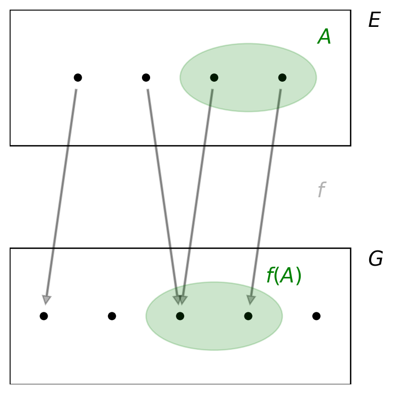
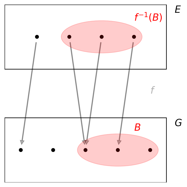
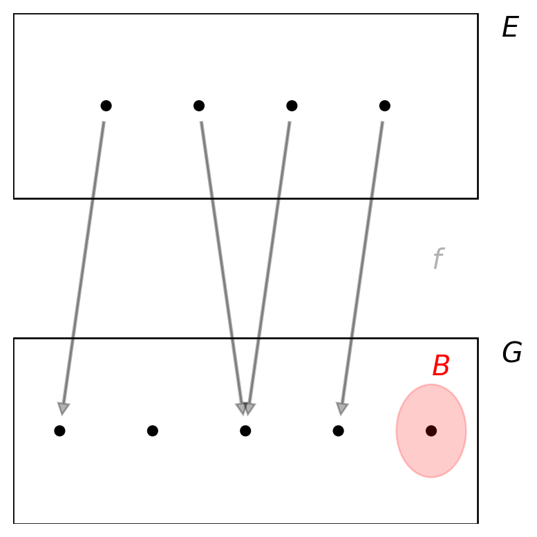
But before going into more detail, let’s recall how a function $f: E \to G$ also naturally maps subsets of $E$ to subsets of $G$ (and vice versa). For any subset $A \subseteq E$, we denote by $f(A)$ the image of $A$ under $f$ i.e. the subset in the codomain $G$ in which all the values are gathered that $f$ visits as it runs through the elements of $A$: \[f(A) := \{ f(x) \, | \, x \in A \} \subseteq G.\] By convention we set $f(\emptyset):=\emptyset$. The inverse image does a similar thing but then the other way around i.e. from codomain back to domain: for any subset in the codomain $B \subseteq G$, you gather all the elements in the domain $E$ that are mapped to a value in $B$ by $f$, i.e. you “map $B$ back to a subset in the domain” if you will. It is denoted by² $f^{-1}(B)$: \[f^{-1}(B) := \{ x \in E \, | \, f(x) \in B \} \subseteq E.\] Note that we naturally have $f^{-1}(\emptyset)=\emptyset$ — it is well possible that for other subsets $B \subseteq G$ we have $f^{-1}(B)=\emptyset$ as well.

² Don’t get confused: you’ll have seen this notation also being used for inverse functions, but this is a different use — whether or not $f$ has an inverse function and what it is is not relevant here. Recall that an inverse function maps individual elements in $G$ back to elements in $E$, and here we are talking about “mapping sets” rather

³ If you’re not entirely sure about any of these, just draw the graph of $f$ in a plot where the horizontal axis represents the domain $\R$ and the vertical axis the codomain $\R$. To determine say $f((-1,3))$, just let $x$ run through the interval $(-1,3)$ on the horizontal axis and keep track of which values on the vertical axis are visited in that process. To determine say $f^{-1}((4,9))$, mark the interval $(4,9)$ on the vertical axis. Then let $x$ run over the horizontal axis and keep track of which values of $x$ get mapped to a value in $(4,9)$. Etc.

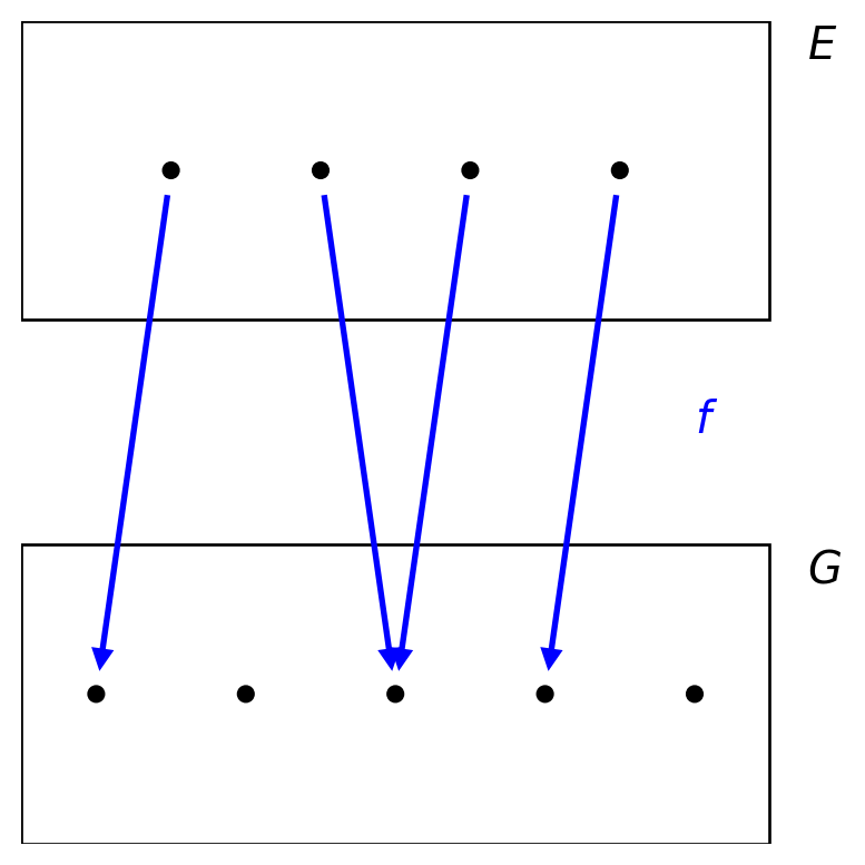
If you like your visuals, then see Figure 2.1 below for illustration (in particular for the countable/finite case). To give a quick example with uncountable sets, take e.g. $E=\R$ and $G=\R$ and consider $f: \R \to \R$ given by $f(x)=x^2$. Then the range of $f$ is $[0,\infty)$ and we have e.g.³ $f([1,2])=[1,4]$, $f((-1,3))=[0,9)$, $f^{-1}((4,9))=(-3,-2) \cup (2,3)$ and $f^{-1}((-\infty,-1])=\emptyset$.

(a) A set/universe $E$ containing four elements, a set/universe $G$ containing five elements, and a function $f: E \to G$ visualised by the blue arrows. Note that the range of $f$ contains three elements

Why would you introduce inverse images when you already have images to work with? Well it turns out that inverse images have certain nice properties that make them more convenient to work with (especially in our context). Here are the key ones (the proof is not very difficult and is left for you to do in Exercise 2.1):

Lemma 2.1 Let $f: E \to G$ be some function. Let $B_1, B_2, \ldots$ be a collection of subsets in $G$. Then:

Taking inverse images can be interchanged with the standard set operations. That is to say, we have for instance: \[f^{-1} \left( \bigcup_{i=1}^\infty B_i \right) = \bigcup_{i=1}^\infty f^{-1}(B_i), \quad f^{-1} \left( B_1^c \right) = \left( f^{-1}(B_1) \right)^c, \quad \text{etc.}\]
If the $B_i$’s form a partition of $G$ (recall from Section 1.2.3), then the collection of subsets $f^{-1}(B_1), f^{-1}(B_2), \ldots$ forms a partition of $E$.

Ok, now that we have reminded ourselves about images and inverse images, we can go back to talking about what we are really interested in: measurability of a function. For our use case, we’ll only really need functions with codomain $G=\R$ and so we’ll focus on functions $f:E \to \R$. Recall that on $\R$, we like to work with the Borel $\sigma$-algebra $\mathcal{B}(\R)$ whose elements we also call Borel sets (cf. Section 1.4). On the domain $E$ we also choose some $\sigma$-algebra, say $\mathcal{F}$. A function $f:E \to \R$ is called measurable if it “plays nicely” with the subset structure these two $\sigma$-algebras give us, in the sense that the inverse image of any Borel set $B$ is an element of $\mathcal{F}$. Note that this property depends both on what function $f$ we pick as well as on what $\sigma$-algebra $\mathcal{F}$ on $E$ we pick: the same function may very well be measure for one $\sigma$-algebra on $E$ but not for another!

Definition 2.1 Let $(E,\mathcal{F})$ be a measurable space (cf. Definition 1.1) and $f:E \to \R$ a function, where on the codomain $\R$ we use the Borel $\sigma$-algebra $\mathcal{B}(\R)$. Then $f$ is called measurable if for any $B \in \mathcal{B}(\R)$ it holds that $f^{-1}(B) \in \mathcal{F}$.

If we want to stress the role of $\mathcal{F}$ (e.g. because we consider multiple $\sigma$-algebras on $E$), then we also use the term $\mathcal{F}$-measurable.

Further, if in the above we have $(E,\mathcal{F})=(\R,\mathcal{B}(\R))$ so that we are in our familiar setting of a function $f: \R \to \R$, then we also use the term Borel measurable (in the literature, this term is more broadly used for any topological space $E$, but we will only use it — and need it — in the case $E=\R$).

Hmm. But does this now mean that if I want to work with some function $f: E \to \R$ and I need it to be measurable, that I need to find a $\sigma$-algebra on $E$ and that I also need to show that it makes $f$ measurable?? :(. Well, in principle yes! But then here’s the good news: the collection of subsets \[\{ f^{-1}(B) \, | \, B \in \mathcal{B}(\R) \}\] is already a $\sigma$-algebra on $E$! This is actually not very hard to see: it relies on the fact that $\mathcal{B}(\R)$ is a $\sigma$-algebra, and that the pleasant way in which $f^{-1}$ interacts with set operations (cf. Lemma 2.1 i) means that the $\sigma$-algebra properties carry over from $\mathcal{B}(\R)$ to this collection.

So this collection/$\sigma$-algebra is the natural one to consider on $E$ to make $f$ measurable. If we already have a $\sigma$-algebra $\mathcal{F}$ on $E$, then it follows that $f$ is $\mathcal{F}$-measurable if and only if $\mathcal{F}$ contains each element in this collection/$\sigma$-algebra i.e. if this collection/$\sigma$-algebra is a sub-$\sigma$-algebra of $\mathcal{F}$.

Definition 2.2 Let $f:E \to \R$ be a function. Consider the collection of subsets $\mathcal{C}$ in $E$ consisting of the inverse images $f^{-1}(B)$ for all Borel sets $B \in \mathcal{B}(\R)$ i.e. \[\mathcal{C}=\{ f^{-1}(B) \, | \, B \in \mathcal{B}(\R) \}. \tag{2.1}\] Then $\mathcal{C}$ is a $\sigma$-algebra on $E$ that we generally denote by $\sigma(f)$ and we call it the $\sigma$-algebra generated by $f$.

Note that, for any given $\sigma$-algebra $\mathcal{F}$ on $E$, $f$ is $\mathcal{F}$-measurable if and only if $\sigma(f) \subseteq \mathcal{F}$.

Remark 2.1. Recall that in Definition 1.2 we first encountered the notation “$\sigma(...)$”, there the “…” had to be a collection of subsets of $E$ and we said that it denotes the $\sigma$-algebra generated by that collection. The above use of $\sigma(f)$ is a natural extension of that: it denotes the $\sigma$-algebra on $E$ generated by all inverse images of Borel sets under $f$ i.e. $\sigma(\mathcal{C})$ with $\mathcal{C}$ given by Equation 2.1. However since $\mathcal{C}$ is already a $\sigma$-algebra we don’t actually need to generate anything i.e. $\sigma(\mathcal{C})=\mathcal{C}$!

Ok, that helps a bit. But listen, what if I have some function $f: E \to \R$ given and also some $\sigma$-algebra $\mathcal{F}$ on $E$, how do I actually practically verify whether or not $f$ is $\mathcal{F}$-measurable? Definition Definition 2.1 would require me to construct the inverse image for any Borel set $B$ (of which there are many as already discussed in Section 1.4) and check that it is an element of $\mathcal{F}$, surely that’s not viable? Well indeed, that’s not very pleasant at first sight! The good news is that some easier to use criterions are available.

Without going into too much detail (we’re a bit at the edge of the scope of our course here, and time is limited of course), here are some of the highlights (don’t worry about having to memorise these, it’s mainly for reference and we’ll use them only rarely explicitly):

Proposition 2.1 Let $(E,\mathcal{F})$ be a measurable space (cf. Definition 1.1) and $f:E \to \R$ a function. Then we have (see e.g. Williams 1991, chap. 3; Stroock 1994, sec. 3.2; Kallenberg 1997, chap. 1):

$f$ is measurable if and only if for any $a \in \R$, $f^{-1}((-\infty,a]) \in \mathcal{F}$. In this statement, you may equally well replace “$(-\infty,a]$” by any of “$(-\infty,a)$”, “$[a,\infty)$” and “$(a,\infty)$”.
If $(E,\mathcal{F})=(\R,\mathcal{B}(\R))$ and $f$ is continuous everywhere with the possible exception of at most countably many points, then $f$ is Borel measurable.
If $f$ is measurable and $g: \R \to \R$ is Borel measurable, then the composition $h=g \circ f$ i.e. $h: E \to \R$ given by $h(x)=g(f(x))$ is measurable.
If $f_1, f_2, \ldots, f_n: E \to \R$ are all measurable, then also any function created from these by “elementary” operations (addition, multiplication, product, division, as well as multiplication with constants) is also measurable.
If $f_1, f_2, \ldots: E \to \R$ are all measurable then so are the functions \[g(x)=\sup_{n \geq 1} f_n(x), \ g(x)=\inf_{n \geq 1} f_n(x), \ g(x)=\begin{cases} \lim_{n \to \infty} f_n(x) & \text{if the limit exists} \\ 0 & \text{otherwise.} \end{cases} \] (in the final expression, the choice for $0$ is arbitrary, it can be any measurable expression).

Some notes:

So, if you want to prove that some given function is measurable, you typically first see whether it is somehow composed/defined in terms of more “elementary” functions. If not, then typically you’d like to use properties i or ii. If it is, then you’d typically like to show that its “elementary” parts are measurable (using property i or ii) and then apply one or more of properties iii–v.
Note that all the constructions in property v are point wise, that is, in each case you fix some $x \in E$ and then take the supremum/infimum/limit of the sequence of real numbers $f_1(x), f_2(x), \ldots$ to construct $g(x)$ (and then repeat that for all other elements in $E$ of course). Recall that any set in $\R$ (hence including such a sequence of real numbers) has a supremum (=smallest upper bound) and infimum (=largest lower bound) although they may be $\infty$ and $-\infty$ respectively. See e.g. Wiki if you’d like a quick refresher.
It is not a coincidence that in i above we again encounter the collection of subsets of $\R$ that was also the focus of our attention in Section 1.6.2!

Remark 2.2. As already transpires a little bit from the final bullet point in Proposition 2.1, there is something slightly dodgy about property v: it is very well possible that a function $g$ as constructed there ends up taking the value $-\infty$ and/or $\infty$, indeed take e.g. $f_n(x)=n$ for all $x \in E$ (is measurable by Exercise 2.3) and $n \geq 1$. Then $g(x)=\sup_{n \geq 1} f_n(x)=\infty$ for all $x \in E$. Now property v seems to claim that this $g$ is measurable, but we haven’t actually defined what that means if the codomain is not just $\R$ but needs to include $\infty$ (and, in other examples, $-\infty$) as well.

For the sake of time, here is a longer story short: you can actually properly (and naturally) handle such functions as well by working with the extended real line as codomain, a measurable space with universe $\R \cup \{-\infty,\infty\}$. The bottom line is that our definition of measurability of a function $g$ on a measurable space $(E,\mathcal{F})$ naturally extends to this case, by just adding the condition that also the inverse images $g^{-1}(\{-\infty\})$ and $g^{-1}(\{\infty\})$ are elements of $\mathcal{F}$ — note that if $g$ only takes values in $\R$ then these two inverse images equal $\emptyset$ and are hence trivially elements of any $\sigma$-algebra (cf. Definition 1.1). See e.g. Stroock (1994) for details if you’re interested.

Example 2.1 The above Proposition 2.1 gives us some tools to attack measurability of functions with in general. There is one special category that is worth briefly highlighting, namely functions $f:E \to \R$ that take only finitely many values i.e. have finite range. Note that if the universe $E$ is a finite set then any function necessarily has finite range, but (of course) such functions also exist on infinite and uncountable universes.

If you think about it for a little bit then you’re probably able to convince yourself that the $\sigma$-algebra $\sigma(f)$ (cf. Definition 2.2) generated by such an $f$ is finite as well. And remember from Example 1.4 that such $\sigma$-algebras are quite nice and easy to understand!

More precisely, if we write the range of $f$ as $\{y_1,y_2,\ldots,y_n\}$, then the sets \[A_1=f^{-1}(\{y_1\}), A_2=f^{-1}(\{y_2\}), \ldots, A_n=f^{-1}(\{y_n\}) \tag{2.2}\] form a partition of $E$ (this is not hard to see independently, it’s also a mild variation of Lemma 2.1 ii). Further, for any Borel set $B$ you can see $f^{-1}(B)$ as follows: check which values in the range of $f$ are part of $B$, and then $f^{-1}(B)$ is exactly the union of the $A_i$’s corresponding to these values. In maths that reads e.g. like \[f^{-1}(B)=\bigcup_{i \in I} A_i, \quad \text{where } I=\{i \in \{1,\ldots,n\} \, | \, y_i \in B \}\] (where we naturally understand $f^{-1}(B)=\emptyset$ if $I=\emptyset$), but it is probably at least as obvious from a visual like in Figure 2.1!

This confirms that $\sigma(f)$ is a $\sigma$-algebra of the type discussed in Example 1.4, where $A_1, \ldots, A_n$ from Equation 2.2 are your atoms.

Finally, note that for any other $\sigma$-algebra $\mathcal{F}$, $f$ is $\mathcal{F}$-measurable if and only if $A_i \in \mathcal{F}$ for all $i=1,\ldots,n$, or, put a bit more loosely: if $\mathcal{F}$ contains all the sets on which $f$ is constant.

Exercises

You can now do Exercise 2.1–Exercise 2.2.

2.3 Probability spaces & random variables

Now we are ready to put all the pieces we have seen so far together and take the perspective that we are most interested in: Probability Theory! This section describes the key mathematical setup that we will be using pretty much all the time in the remainder of this course, so it’s really important to make sure you digest and understand it well!

Recall that all things Probability Theory start from some random experiment for which we want to build a mathematical model so that we can analyse it. In order to do so, we start by collecting all possible outcomes of the experiment we are interested in in a set/universe that we like to call the outcome space (or sample space) and typically denote by $\Omega$. Commonly we use the symbol $\omega$ when we talk about possible outcomes/elements of the outcome space, but that’s merely a convention.

Further we typically want to measure something specific about the possible outcomes, which we do by means of a function/mapping $X: \Omega \to \R$. For example, suppose that we toss two coins and are interested in the number of heads we get. Then we can for instance choose $\Omega=\{TT,TH,HT,HH\}$ with $X: \Omega \to \R$ given by $X(TT)=0$, $X(TH)=X(HT)=1$ and $X(HH)=2$. Note that $X$ can very well be a rather trivial function. For instance if we want to model rolling a die, we could simply take $\Omega=\{1,\ldots,6\}$ and let $X: \Omega \to \R$ be the identity mapping i.e. $X(1)=1$, $X(2)=2$, …, $X(6)=6$. It’s just convenient to always use such functions to get the end result we are interested in, even if they don’t actually do a lot, as we’re then always working in the same context.

Of course, as we know from earlier Probability courses, there are two more key ingredients that we need: events and probabilities. Events are subsets of $\Omega$ i.e. sets containing some (or none in case of the empty set) possible outcomes of the experiment, and an event can occur (or: happen) or not: it occurs/happens if we run the experiment and the outcome we observe is an element of the event. There are two “extreme” events: $\Omega$ itself is an event that is guaranteed to happen (after all, whenever you do the experiment you necessarily get an outcome from $\Omega$) while the empty set $\emptyset$ is an event that never happens. Further we like to assign probabilities to events: each event is assigned a number from $[0,1]$ that quantifies how likely the event is to occur if we run the experiment once.

So our mental model of a random experiment is: you execute it, observe a certain outcome say $\omega \in \Omega$, and then plug that outcome into your $X$ to observe a value $X(\omega) \in \R$ (we also like to call this the value that $X$ takes). Note that hence, before you run the experiment, you do not yet know what outcome you’ll get to observe and neither what value $X$ ends up taking. There is a fundamental link between this empirical perspective and the modelling perspective in which you specify probabilities of events: if you fix some event, run the experiment $n$ times and count how often the event occurs, say $k(n)$, then as $n \to \infty$ the relative frequency $k(n)/n$ converges to the probability of the event⁴ — of course this is nothing but the good old Law of Large Numbers. In fact, this is how you would determine/define the probabilities of the events in your model if you started from an empirical perspective. I know that this paragraph seems almost too obvious to write down, and maybe it is, but as we go forward to develop increasingly convoluted theoretical layers on this basis it can be really helpful at times to think back to this mental model!

⁴ Of course, we actually create that link by choosing our probabilities accordingly (if your starting point is truely a physical experiment) or by choosing an appropriate experiment (if your starting point is a model i.e. an $\Omega$ with given probabilities for events). This relationship won’t be there if you use the model for a fair die and apply it to an experiment in which you actually roll a non-fair die for instance!

Now, let’s link this back to the work we have done in Chapter 1 and Section 2.2 above. As we’ve discussed previously (cf. Remark 1.3), we can’t (generally) take all subsets of $\Omega$ to be valid events without running into technical trouble with properly definining probabilities. So we need to settle for choosing a $\sigma$-algebra $\mathcal{F}$ on $\Omega$ and consider only elements of $\mathcal{F}$ to be our events. This makes $(\Omega,\mathcal{F})$ a measurable space. Further to make the notion of probabilities of these events precise, we use a measure on $\mathcal{F}$ for which we typically use the symbol “$\P$” (rather than a “$\mu$” as we used previously for general measures) with the property that $\P(\Omega)=1$ ($\Omega$ is guaranteed to be an event, no matter what $\sigma$-algebra we decide to use (cf. Exercise 1.1) and it is an event that trivially always occurs). This makes the triplet $(\Omega,\mathcal{F},\P)$ nothing but a measure space containing in particular a probability measure.

Finally, for the mapping $X:\Omega \to \R$ we mentioned above, we impose the condition that it is measurable with respect to the above $\sigma$-algebra $\mathcal{F}$ and then we call it a random variable. This ensures that we can do the following. Recall from the above mental model, we can imagine executing the expriment once and (ultimately) observing that $X$ takes a certain value in $\R$. This naturally brings up the following question: if we fix some subset $B \subseteq \R$ and execute the experiment once, what is the probability that $X$ takes a value in $B$? For example, if $X$ is the result of rolling a die, what is the probability that $X$ is larger than $3$ (i.e. takes a value in $(3,\infty)$)? Note that by very definition of the inverse image (as discussed above in Section 2.2), $X$ takes a value in $B$ if and only if the outcome of the expriment is an element of the event $X^{-1}(B) \subseteq \Omega$ i.e. if the event $X^{-1}(B)$ occurs (note it is an event i.e. element of $\mathcal{F}$ due to our measurability condition on $X$, provided that $B$ is a Borel set).

So, in conclusion the above paragraph tells us: for a random variable $X$ and Borel set $B$, the probablity that $X$ takes a value in $B$ is naturally understood/defined as the probability of the event $X^{-1}(B)$ i.e. $\P(X^{-1}(B))$, via the following two-step process: \[B \in \mathcal{B}(\R) \quad \stackrel{X^{-1}}{\longrightarrow} \quad X^{-1}(B) \in \mathcal{F} \quad \stackrel{\P}{\longrightarrow} \quad \P(X^{-1}(B)) \in [0,1].\]

Because computing probabilities involving random variables like the above is such a common thing, over time people have got a bit lazy with notation. The event $X^{-1}(B)$ can also be written as $\{ \omega \in \Omega \, | \, X(\omega) \in B \}$ and this is often lazily abbreviated to just “$\{ X \in B\}$” or a variation thereof. E.g. “$\{ X>3\}$” is shorthand for the event \[\{ \omega \in \Omega \, | \, X(\omega) >3 \}=X^{-1}((3,\infty)).\] Further, when used as argument in a probability measure, we typically even drop the curly brackets i.e. we tend to write “$\P(X>3)$” to actually mean $\P(\{ \omega \in \Omega \, | \, X(\omega) >3 \})$ or, equivalently, $\P(X^{-1}((3,\infty)))$. Of course, if you’re not too comfortable with the shorthand, it’s always fine to use the full form as well. Otherwise please always try to read such expressions carefully and keep the following in mind: since $\P$ is a mapping from $\mathcal{F}$ to $[0,1]$, whatever appears as argument in $\P$ must always be an event i.e. element of $\mathcal{F}$ (in shorthand form or otherwise).

Remark 2.3. Note that Proposition 2.1 is quite handy to construct new random variables from existing ones without any hard work. For instance, if $X$ is a random variable then so is $Y=X^2$, by which we (of course) mean the function $Y: \Omega \to \R$ given by $Y(\omega)=X(\omega)^2$ for all $\omega \in \Omega$. Since this is the composition of the measurable function $X: \Omega \to \R$ (as it’s a random variable) and the continuous function $g:\R \to \R$ given by $g(x)=x^2$, it follows from Proposition 2.1 ii & iii that $Y$ is measurable as well and hence a random variable. We’ll use this argument regularly going forward (often without explicitly pointing this out).

Let’s conclude this section by putting the key points together, then Figure 2.2 below in which the key points of this section are visualised, and finally some examples.

Definition 2.3 Our mathematical model for a random experiment consists of a measure space (cf. Definition 1.3) $(\Omega,\mathcal{F},\P)$ consisting of a universe $\Omega$ containing all the possible outcomes of the experiment, a $\sigma$-algebra $\mathcal{F}$ on $\Omega$ whose elements are the subsets of $\Omega$ that we consider to be events, and $\P:\mathcal{F} \to [0,1]$ a measure that maps an event $A$ to $\P(A) \in [0,1]$ representing the likelihood that $A$ occurs/happens if we execute the experiment once. Further $\P$ has the property that $\P(\Omega)=1$ which makes it a probability measure. We call $(\Omega,\mathcal{F},\P)$ a probability space.

Note that (of course) all the previously established properties for measure spaces apply (it’s just that in Probability Theory it’s common to write “$\Omega$” rather than “$E$” and “$\P$” rather than “$\mu$”), in particular $\P$ satisfies the properties we listed in Definition 1.3 and Theorem 1.1.

Further a random variable is an $\mathcal{F}$-measurable function $X: \Omega \to \R$ (cf. Definition 2.1). We like to use shorthand notation for (probabilities of) inverse images of $X$, see the above discussion.

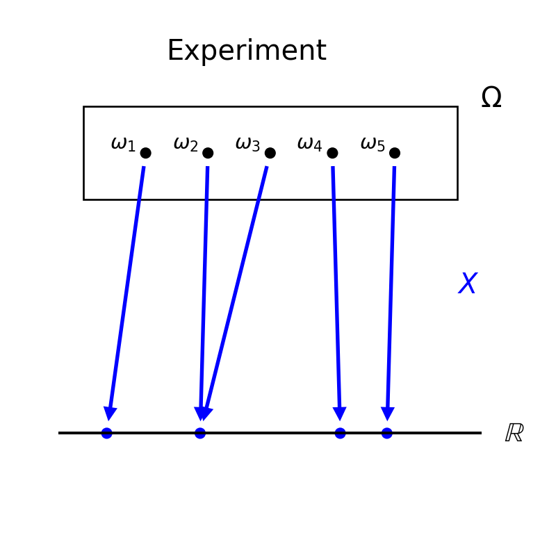
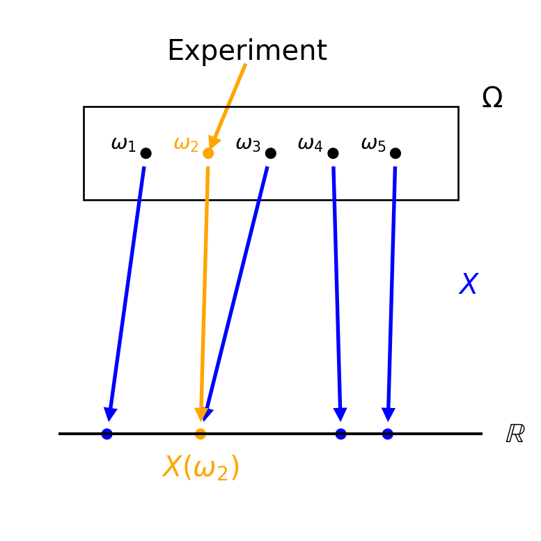
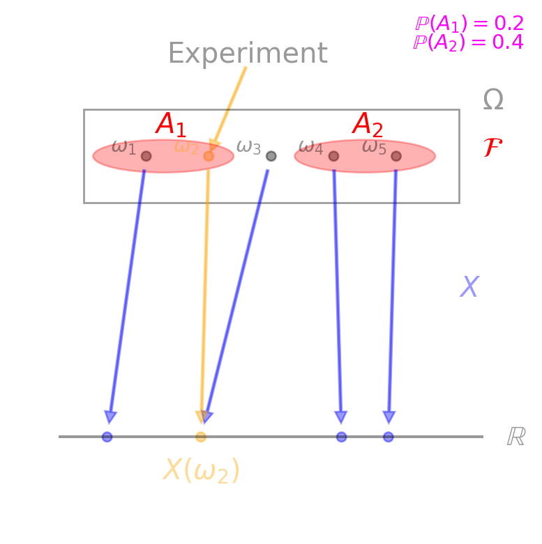
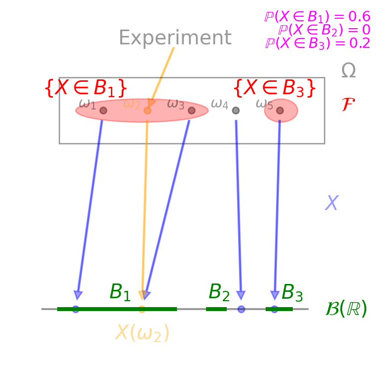
(a) The basic setup: a random experiment whose possible outcomes are collected in $\Omega$, and a random variable $X: \Omega \to \R$

Example 2.2 Here are some examples of random experiments and how they could be translated into probability spaces and random variables. Recall that in the case of a countable $\Omega$, we can simply choose the powerset of $\Omega$ as our $\sigma$-algebra and define a probability measure $\P$ by assigning probabilities to the elements of $\Omega$ (as singletons), cf. Remark 1.3.

We toss two (fair) coins twice and are interested in the number of heads we get (as already encountered in the text above). Then we can for instance choose $\Omega=\{TT,TH,HT,HH\}$. Since we are in the countable case we can simply set $\mathcal{F}=\mathcal{P}(\Omega)$, and our probability measure $\P$ is defined on the singletons by setting \[\P(\{TT\})=\P(\{TH\})=\P(\{HT\})=\P(\{HH\})=\frac{1}{4}.\] Further we define $X: \Omega \to \R$ by setting $X(TT)=0$, $X(TH)=X(HT)=1$ and $X(HH)=2$. We would intuitively expect that the probability of getting one head to be equal to $1/2$. Here is how we could verify this formally in this setup, with the shorthand notation discussed earlier in this section: \[\text{Prob one head}=\P(X=1)=\P(\{TH,HT\})=\P(\{TH\})+\P(\{HT\})=\frac{1}{2},\] where we use that $\{X=1\}=X^{-1}(1)=\{TH,HT\}$ and countable additivity (cf. Definition 1.3) for the third equality.
We roll $n$ fair dice and are interested in the sum of the eyes. The outcome space naturally consists of all length $n$ sequences of numbers from $1,2,\ldots,6$, which we could e.g. write as \[\Omega=\{ \omega=(\omega_1,\omega_2,\ldots,\omega_n) \, | \, \omega_i \in \{1,2,\ldots,6\} \text{ for all } i=1,2,\ldots,n \}.\] Since we are still in the countable case ($\Omega$ is finite after all, containing $6^n$ elements) we can again use the powerset for our $\sigma$-algebra and since all outcomes are equally likely, define our probability measure $\P$ on the singletons by setting \[\P(\{\omega\})=\frac{1}{6^n} \quad \text{for all $\omega \in \Omega$}.\] Further we should define $X: \Omega \to \R$ as \[X(\omega)=\sum_{i=1}^n \omega_i.\] Note that since we can write any event $A$ as a (finite) union of its elements as singletons and all these singletons have probability $1/6^n$, countable additivity brings us to \[\P(A)=\frac{|A|}{6^n},\] where $|A|$ denotes the number of elements in $A$. (Of course this works in general for any experiment with finitely many equally likely outcomes, including the two coins example above).
We roll infinite many fair dice. In this situation we would naturally choose, as extension of the previous example \[\Omega=\{ \omega=(\omega_1,\omega_2,\ldots) \, | \, \omega_i \in \{1,2,\ldots,6\} \text{ for all } i=1,2,\ldots \}\] i.e. all infinite sequences whose entries are numbers from $1$ to $6$. There is however a serious difference with the previous case: now $\Omega$ is uncountable (cf. Section 1.2.1) and hence we can no longer use these “simple” principles as we used in the previous two examples, we now have to put some serious thought and work into constructing a suitable $\sigma$-algebra and probability measure!
Choose a real number from the interval $[0,1]$ at random, where each number is equally likely. Now, the ‘equally likely’ wording here is a bit deceptive as it may make you think back to the “simple” second example above. However the natural choice is now $\Omega=[0,1]$ which is again uncountable (cf. Section 1.2.1)… We would be equally stuck as in the previous example, if we hadn’t yet already encountered our saviour before! Indeed recall the Lebesgue measure $\lambda$ from Proposition 1.2 — we could choose $\mathcal{F}=\mathcal{B}([0,1])$ and $\P=\lambda$ (restricted to $[0,1]$). We know already that $\lambda$ (and hence $\P$) is a measure, and since \[\P(\Omega)=\P([0,1])=\lambda([0,1])=1-0=1,\] $\P$ is indeed a probability measure. So with these choices, $(\Omega,\mathcal{F},\P)$ is indeed a valid probability space according to Definition 2.3. However is it also the “right” choice i.e. does it (in particular the probability measure) reflect the experiment that we have in mind? Well the truth is that we first have to admit that “equally likely” does not make any real sense in this context, it only makes literal sense in a finite context. We can mimick the finite case by thinking in terms of intervals in $[0,1]$ rather than individual real numbers. If you think about it, then you can rephrase the intended meaning of “equally likely” as “any two intervals in $[0,1]$ of equal length are equally likely to contain the number that gets chosen” right? And since the Lebesgue measure of an interval equals its length, that condition is indeed satisfied by our choices.

2.4 Almost sure (a.s.) events

In this short section we highlight one particular aspect of our setup that will be used regularly going forward. As discussed, in the context of a probability space $(\Omega,\mathcal{F},\P)$, we express how likely an event $A$ is to occur by means of its probability $\P(A) \in [0,1]$. The largest possible value is $1$ so in that case the event is as likely to happen as it gets. You could be forgiven for expecting that that means that such an event must happen with absolutely certainty each time we execute the experiment.

Note that the only event that is absolutely certain to happen is $\Omega$ itself — after all, no matter what outcome $\omega \in \Omega$ the experiment yields, it is trivially an element of $\Omega$. And generally, in the simple case of a probability space with a finite $\Omega$, the probability measure is (or: can be) chosen so that $\Omega$ is the only event with probability $1$ and you have the association “event is guaranteed to happen $\leftrightarrow$ event has probability $1$”.

However this association is typically no longer valid if $\Omega$ is has infinitely many elements. For example, think back to our model for choosing a number from the interval $[0,1]$, all numbers “equally likely”, as discussed in Example 2.2 iv. Consider the event $A=[0,1/2) \cup (1/2,1]$. Then, using countable additivity (cf. Definition 1.3) \[\P(A)=\lambda(A)=\lambda([0,1/2))+\lambda((1/2,1])=1/2-0+1-1/2=1\] so $A$ has probability $1$ but $A$ is not guaranteed to happen, after all it could be that the outcome of our experiment is $\omega=1/2$.

In a lot of the work we’ll be doing, we’ll encounter statements that we know/can prove to be true only on an event with probability $1$, but not (necessarily) “absolutely certain” i.e. for any $\omega \in \Omega$. Therefore it is convenient to have a short way of pointing this out, and that’s where the phrase almost surely comes in⁵.

⁵ In the more general measure theory context we considered in Chapter 1, commonly the term “almost everywhere (a.e.)” is used

Definition 2.4 On a probability space $(\Omega,\mathcal{F},\P)$ (cf. Definition 2.3), an event $A$ is said to happen almost surely (a.s.), or sometimes $\P$-almost surely ($\P$-a.s.) if we want to stress the role of $\P$, if it has probability $1$ i.e. $\P(A)=1$.

Exercises

You can now do Exercise 2.4–Exercise 2.5.

2.5 The law/distribution of a random variable

In Section 2.3 we were insisting that in order to model a random experiment, we need a probability space and (typically) a random variable. Ok. But then, you’ll remember from your earlier Probability courses that quite often an example/exercise/… started with a statement like “Let $X$ be a random variable with a Poisson distribution with parameter $1$.” and you went on to compute things like probabilities for $X$, its mean, variance or other moments, moment generating function, characteristic function or any other of the whole load of distributional properties that you have encountered in the past. Somehow we could do such computations without actually having to talk about/specify the probability space on which $X$ was defined… How does that even work??

The answer to this apparent conundrum comes in two parts:

Part 1: given a full setup of a probability space and a random variable $X$ as discussed in Section 2.3, to study distributional properties of $X$ such as the ones mentioned above, we only need to know “how $X$ behaves on the real line” (visually, the real line in Figure 2.2 i.e. the codomain of $X$) — roughly speaking, what values $X$ takes there and with what probabilities that happens⁶. That behaviour can be described by means of a concept called the law or distribution of $X$. So all we really need to do is to extract the law/distribution of $X$ from the whole setup and then we are ready to answer any questions related to the distributional properties of $X$.
Part 2: it can be shown that given any law/distribution you are particularly interested in, you can always construct a full setup consisting of a probablity space and random variable $X$ such that $X$ has indeed the law/distribution you are interested in. So if all we need is a random variable with a certain given law/distribution then we know that we can construct a full setup for it but we just can’t be bothered to do that (or even to point that out!). So a statement like “Let $X$ be a random variable with a Poisson distribution with parameter $1$.” is actually shorthand for “Let $X$ be a random variable with a Poisson distribution with parameter $1$, defined on a probability space that we know we can construct but is not relevant for our interests here so we don’t bother even mentioning it.”.

⁶ This description is only literally accurate if $X$ is a discrete random variable

In this section, we’ll dig out this concept of a law/distribution of a random variable and address both parts above while we’re at it. Let’s start with Part 1. Given some probability space $(\Omega,\mathcal{F},\P)$ on which a random variable $X: \Omega \to \R$ lives, recall from Section 2.3 that for any Borel set $B$ we can naturally define/understand \[\text{Prob that $X$ takes its value in $B$}=\P(X \in B)\] (which, recall, is shorthand for $\P(X^{-1}(B))$). We can capture this association as a mapping denoted by $\mu_X$, i.e. $\mu_X: \mathcal{B}(\R) \to [0,1]$ given by \[\mu_X(B)=\P(X \in B)=\P(X^{-1}(B))=\text{Prob that $X$ takes its value in $B$} \in [0,1]. \tag{2.3}\] We think about this mapping as encoding/describing everything there is to know about how $X$ behaves on its codomain the real line i.e., loosely speaking, what values $X$ takes and with what probabilities. That’s its key purpose for us. Nevertheless, if we look at it with a cool mathematical eye and analyse it, it has some fascinating properties: it is in fact a measure, even a probability measure (as defined in Definition 1.3) on the measurable space $(\R,\mathcal{B}(\R))$ (cf. Exercise 2.6). So with the introduction of $\mu_X$, the codomain of $X$ effectively gets upgraded from the measurable space $(\R,\mathcal{B}(\R))$ to a probability space $(\R,\mathcal{B}(\R),\mu_X)$.

We call $\mu_X$ the distribution or law of $X$:

Definition 2.5 Let $X: \Omega \to \R$ be a random variable on a probability space $(\Omega,\mathcal{F},\P)$ (cf. Definition 2.3). Then the probability measure $\mu_X$ on $(\R,\mathcal{B}(\R))$ defined by Equation 2.3 is called the distribution (or law) of $X$.

Remark 2.4. If you like your visuals, then make sure to see the above in the context of Figure 2.2 (d). Note that (all) that happens here is that we map the Borel sets on the real line (the ones in green) to the probabilities (in magenta) of the inverse image (in red) corresponding to the Borel set. So, in particular, for the example Borel sets listed there, we get that $\mu_X(B_1)=0.6$, $\mu_X(B_2)=0$ and $\mu_X(B_3)=0.2$. Now imagine that you execute this same process for any Borel set you could put in that real line (in green) to map it to a number: that is your visual image of what $\mu_X$ is doing!

The distribution of $X$ contains all the information you need to compute any distributional property⁷ of $X$ like the ones mentioned earlier. And so if we are only interested in such properties, we only need to keep $\mu_X$ and can forget about the probability space and even the mapping $X$ itself! (However be aware that they of course do determine what $\mu_X$ exactly looks like in a given situation, for instance if we were to replace the probability measure $\P$ by another one, say $\Q$, then as Equation 2.3 shows this will generally result in a different distribution $\mu_X$ because then generally $\Q(X \in B) \not= \P(X \in B)$!)

⁷ Of course this is in a way a circulair definition: a property of $X$ is “distributional” if it only depends on the law/distribution of $X$

Let’s look at a quick example to see a distrbution in action:

Example 2.3 Consider two simple experiments: experiment 1 is flipping a single (fair) coin and we let $X_1$ be $0$ or $1$ depending on whether we get a heads or not, and experiment 2 is rolling a (fair) die and we let $X_2$ be $0$ or $1$ depending on whether we get an even or odd number.

If we write down the full setup for each experiment (keeping in mind that both are “simple” and hence for the probability measure, it is enough to specify it on singletons only as seen before in Example 2.2 e.g.), we could e.g. choose for experiment 1 \[\Omega_1=\{H,T\}, \quad \mathcal{F}_1=\mathcal{P}(\Omega_1), \quad \P_1(\{T\})=\P_1(\{H\})=\frac{1}{2}\] and $X_1: \Omega_1 \to \R$ given by $X_1(T)=0$ and $X_1(H)=1$; while for experiment 2 we could choose \[\Omega_2=\{1,\ldots,6\}, \quad \mathcal{F}_2=\mathcal{P}(\Omega_2), \quad \P_2(\{1\})=\P_2(\{2\})=\ldots=\P_2(\{6\})=\frac{1}{6}\] and $X_2: \Omega_2 \to \R$ given by $X_2(2)=X_2(4)=X_2(6)=0$ and $X_2(1)=X_2(3)=X_2(5)=1$. We have now two separate probability spaces and random variables: $(\Omega_1,\mathcal{F}_1,\P_1)$ with $X_1$ for experiment 1 and $(\Omega_2,\mathcal{F}_2,\P_2)$ with $X_2$ for experiment 2.

However, if we focus only on what happens on the real line (think e.g. about each experiment visualised as in Figure 2.2 (d)) then we see no difference between these experiments at all: both $X_1$ and $X_2$ have as possible values only $0$ and $1$, and it is straightforward to check that they take these values with the same probabilities as well: \[\P(X_1=0)=\P(X_1=1)=\frac{1}{2} \quad \text{and} \quad \P(X_2=0)=\P(X_2=1)=\frac{1}{2}.\] If you are an ant living on the real line and have no idea of what is happening above you (in the visual of Figure 2.2), then all you know is this: each time you hear somebody shout “Experiment executed SIR!”, then either the number $0$ lights up or the number $1$ lights up and that these are equally likely to happen, irrespective of whether experiment 1 or experiment 2 was executed!

We see this equivalent behaviour of both random variables on the real line also reflected in their distributions: if you think about it for a moment, then if you work out $\mu_{X_1}$ and $\mu_{X_2}$ then you find the same result for both, namely the probability measure on $(\R,\mathcal{B}(\R))$ specified by (convince yourself!!), for any Borel set $B$ \[\mu_{X_1}(B)=\mu_{X_2}(B)=\begin{cases} 0 & \text{if $0 \not\in B$ and $1 \not\in B$} \\ 1/2 & \text{if either $0 \in B$ and $1 \not\in B$, or $0 \not\in B$ and $1 \in B$} \\ 1 & \text{if $0 \in B$ and $1 \in B$.} \end{cases} \tag{2.4}\] If you have trouble seeing this, then note that we’re using $\mu_{X_i}(B)=\P(X_i \in B)$ (cf. Equation 2.3), and that since $X_i$ takes only the values $1$ and $2$, for every Borel set $B$ we only care whether or not it contains $1$ or $2$, or neither, or both. If for instance $B$ is such that $0 \not\in B$ and $1 \in B$, then we get that $\{ X_i \in B\}=\{ X_i=1\}$ and hence $\mu_{X_i}(B)=\P(X_i=1)=1/2$. It can also be very helpful to make a sketch for yourself of what Figure 2.2 (d) looks like in either experiment 1 or experiment 2 (or both) — all we’re doing here is work out the maths as directly implied by that visual!

The above example shows that two random variables defined on different probability spaces (or the same probability space) can very well have the same distribution, in which case all their distributional properties are (of course) identical as well.

As the final step in our discussion of Part 1 above, let’s wonder about the following. We have now properly defined what the distribution of a random variable looks like mathematically. However it probably doesn’t really look like what you would have expected — I mean, from your earlier Probability courses you’ll associate “the distribution of a random variable” likely with having a probability mass function (pmf) or a probability density function (pdf) to work with. Or, indeed, a cumulative distribution function (cdf): you may remember from your earlier Probability courses that you were told that any random variable has a cdf (while pmf’s and pdf’s are specific for discrete and continous random variables resp., we’ll get back to these in a little bit). Let’s quickly recall:

Definition 2.6 Let $X: \Omega \to \R$ be a random variable on a probability space $(\Omega,\mathcal{F},\P)$ (cf. Definition 2.3). Then the function $F_X:\R \to [0,1]$ defined by $F_X(x)=\P(X \leq x)$ for all $x \in \R$ is called the cdf of $X$. It has the following properties:

it is non-decreasing and right-continuous (recall the first comment in Lemma 1.2),
it has limit $0$ for $x \to -\infty$ and limit $1$ for $x \to \infty$.

How do we marry up our work so far (distributions as specified by Definition 2.5) with the old stuff that tells us to use cdf’s to talk about distributions? Well indeed, this is where our beautiful Lemma 1.2 comes in! Given a random variable $X$ on a probability space $(\Omega,\mathcal{F},\P)$ with distribution $\mu_X$, Lemma 1.2 tells us that $\mu_X$ (keeping in mind that it is a probability measure i.e. $\mu_X(\R)=1$) uniquely corresponds to one function $F:\R \to [0,1]$ satisfying properties i and ii in Definition 2.6, namely the one given by $F(x)=\mu_X((-\infty,x])$ for all $x \in \R$. Plugging in the def of $\mu_X$, we can work this out to \[F(x)=\mu_X((-\infty,x])=\P(X^{-1}((-\infty,x]))=\P(X \leq x) \quad \text{for any $x \in \R$} \tag{2.5}\] i.e. this $F$ is exactly the cdf $F_X$ of $X$!

So, bottom line: to (uniquely) specify the distribution of the random variable $X$ (in the context of all possible distributions random variables can have), we can either work with $\mu_X$ (in the context of all probability measures on $(\R,\mathcal{B}(\R))$) as defined in Definition 2.5, or we can work with its cdf $F_X$ (in the context of all functions $F:\R \to [0,1]$ satisyfing properties i and ii in Definition 2.6).

Example 2.4 Let’s work out the cdf, say $F$, corresponding to the distribution of $X_1$ (as well as $X_2$) from Example 2.3. That is, the function $F: \R \to [0,1]$ given by $F(x)=\P(X_1 \leq x)$ for all $x \in \R$. For clarity, let’s do this in two ways: once using the expression for $\mu_{X_1}$, and once directly using our knowledge of $X_1$ as you would have done it in your earlier Probability courses (i.e. not using $\mu_{X_1}$).

For the first way, we use $F(x)=\mu_{X_1}((-\infty,x])$ with $\mu_{X_1}$ as given in Equation 2.4. We imagine letting $x$ run from $-\infty$ to $\infty$.

For any $x<0$, $(-\infty,x]$ contains neither $0$ nor $1$ and hence we get from Equation 2.4 with $B=(-\infty,x]$ that $F(x)=0$ (top case).
For any $x \in [0,1)$ we get from Equation 2.4 with $B=(-\infty,x]$ that $F(x)=1/2$ (middle case).
Finally for any $x \geq 1$ we get from Equation 2.4 with $B=(-\infty,x]$ that $F(x)=1$ (bottom case).

For the second way, we use $F(x)=\P(X_1 \leq x)$ and that we have seen in Example 2.3 that $X_1$ takes two values, namely $1$ and $2$, each with probability $1/2$. Again we imagine letting $x$ run from $-\infty$ to $\infty$. (Note that also the arguments used here can be seen straightforwardly from a visual like Figure 2.2 (d)!)

For any $x<0$, it cannot happen that $X_1 \leq x$ (since the possible values are $0$ and $1$) and hence the prob that this happens is simply $0$ i.e. $F(x)=0$ (more technically: $\{ X_1 \leq x\}=\emptyset$ and hence $\P(X_1 \leq x)=\P(\emptyset)=0$ by Definition 1.3).
For any $x \in [0,1)$, $X_1 \leq x$ holds if $X_1$ takes the value $0$ but not if it takes the value $1$. Hence the prob that that this happens equals the prob that $X_1$ equals $1$ i.e. $1/2$, so $F(x)=1/2$ (more technically: $\{ X_1 \leq x\}=\{X=1\}$ and hence $\P(X_1 \leq x)=\P(X=1)=1/2$).
Finally for any $x \geq 1$, $X_1 \leq x$ is guaranteed to happen (no matter whether $X_1$ takes the value $0$ or $1$) and therefore $F(x)=1$ (more technically: $\{ X_1 \leq x\}=\Omega$ and hence $\P(X_1 \leq x)=\P(\Omega)=1$ by Definition 2.3).

In conclusion, both routes (reassuringly) lead to the same cdf for $X_1$, namely \[F(x)=\begin{cases} 0 & \text{if $x<0$} \\ 1/2 & \text{if $x \in [0,1)$} \\ 1 & \text{if $x \geq 1$.} \end{cases} \] Good to double check: indeed non-decreasing, right-continuous and with the right limits (cf. Definition 2.6), as it should be!

This wraps up our discussion of Part 1 above, let’s now move on to Part 2. We can actually also argue the other way around! Let’s start with fixing any distribution i.e. with fixing any probability measure $\mu$ on $(\R,\mathcal{B}(\R))$ or, equivalently, fixing any function $F:\R \to [0,1]$ satisyfing properties i and ii in Definition 2.6. Then the claim of Part 2 is that a probability space $(\Omega,\mathcal{F},\P)$ with random variable $X: \Omega \to \R$ exists so that $X$ indeed has the distribution we had fixed (i.e. so that $\mu_X=\mu$ or equivalently $F_X=F$). We’ll leave this for you to think about in Exercise 2.7!

Remark 2.5. Note that all the distributions you know by name from your earlier Probablity courses (Poisson, Binomial, Exponential, Normal, …) are “just” specific examples of a distribution i.e. a probability measure $\mu$ on $(\R,\mathcal{B}(\R))$ (or a cdf). They are not special in any way other than that they tend to pop up a lot in particular applications/uses or are have some particularly appealing properties, and therefore have gained the privilige over time to become known by a specific name. For example, the distribution of both $X_1$ and $X_2$ in Example 2.3 you know well by its name, it is the good old Bernoulli distribution (with parameter $1/2$)!

Exercises

You can now do Exercise 2.6–Exercise 2.9.

2.5.1 Discrete vs continuous vs ‘other’ random variables

Now we have firmly established what the distribution of a random variable is, let’s talk a little bit more about the different types of random variables/distributions we can have — as you’ll already have seen in earlier Probability courses, but it is good to briefly reiterate this in our current context, and it is also a good point of departure for the next chapter! If you’re interested in a more precise story around these different cases, see Section 4.7.3.

Let $X: \Omega \to \R$ be a random variable on a probability space $(\Omega,\mathcal{F},\P)$. Since $X$ is also “just” a (measurable) function, recall from Section 2.2 that it has a range i.e. the set of values on the real line (its codomain) that gets visited by $X$ as we walk through all $\omega \in \Omega$: \[\{ X(\omega) \, | \, \omega \in \Omega \} \subseteq \R.\]

We’ll see here again the faultline of countable vs uncountable (recall from Section 1.2.1) that we have run into multiple times before already: as long as the range of $X$ is countable everything is nice and “simple”, but if we go beyond that things become a lot more “advanced”!

We say that $X$ is a discrete random variable if its range is countable, let’s write it as $\{x_1, x_2, \ldots\} \subseteq \R$ (could be finite as well of course). In this case its distribution (as defined in Definition 2.5) is fully determined by the values that $\mu_X$ assigns to the singletons $\{x_1\}, \{x_2\}, \ldots$ (and $\mu_X$ effectively boils down to the well known probability mass function (pmf)): for any Borel set $B$, check for which $i=1,2,\ldots$ we have $x_i \in B$ and then $\mu_X(B)$ is just the sum of the $\mu(\{x_i\})$’s for the relevant $i$’s.

Further recall from your earlier Probability courses that the cdf of a discrete $X$ takes the form of a piecewise constant function, whose jumps/discontinuities happen at each of the $x_1, x_2, \ldots$ and their sizes are $\mu(\{x_1\}), \mu(\{x_2\}), \ldots$. Also you’ll remind the following standard formula for the expectation of any (Borel measurable, recall Remark 2.3) function $h:\R \to \R$ of $X$: \[\E[h(X)]=\sum_{i=1}^\infty h(x_i) \mu(\{x_i\}) = \sum_{i=1}^\infty h(x_i) \P(X=x_i) \tag{2.6}\] (provided that this sum exists). Note that this has a nice interpretation: it is a weighted average of the values that $h(X)$ takes i.e. $h(x_1), h(x_2), \ldots$ weighted with the corresponding probabilities that $h(X)$ ends up in each of these values. This concept will be a source of inspiration in Chapter 3!

Now let’s move beyond the realm of “simple” discrete random variables and consider a random variable $X$ with uncountable range (note that this means that necessarily, $\Omega$ is uncountable as well). Of those, from earlier Probability courses we only understand a specific subclass, namely the continuous random variables, those whose cdf $F_X$ can be expressed as follows: \[F_X(x)=\int_{-\infty}^x f_X(y) \d y \quad \text{for all $x \in \R$,} \tag{2.7}\] where $f_X$ is an (integrable) function $f_X: \R \to [0,\infty)$ called the probability density function (pdf) of $X$. Note that Equation 2.7 ensures that $F_X$ is at least absolutely continuous (slightly more smooth than continuous, see e.g. Wiki).

To be fully precise, to use these Equation 2.7 to its fullest extent we should be using Lebesgue integration — which we’ll run into in the next chapter! Further note that for the distribution $\mu_X$ of $X$ (as defined in Definition 2.5), we get from Equation 2.5 that \[\mu_X((-\infty,x])=F_X(x)=\int_{-\infty}^x f_X(y) \d y \quad \text{for all $x \in \R$,}\] which gives a glimpse of the very interesting fact that the pdf $f_X$ can be naturally interpreted as a “density” that $\mu_X$ has with respect to the Lebesgue measure (and which we can be pursued in a more general measure theoretic context as well) — however here we are bouncing into the edge of the scope of our course/what we have time for, if you’re interested in more details then see Section 4.7.3.

You’ll also remember from your earlier Probability courses that in this situation, we also have a nice formula for the expectation of any (Borel measurable) function $h:\R \to \R$ of $X$: \[\E[h(X)]=\int_{-\infty}^\infty h(y) f_X(y) \d y \tag{2.8}\] (provided the integral exists — and again the Lebesgue integration comment applies).

Remark 2.6. Here are two quick asides — nothing crucial but “while we’re talking about this anyway” type of stuff.

In the context of a continuous random variable $X$, we often talk about “the pdf of $X$”. However this is a bit deceiving, indeed the pdf is not unique! For instance, if $f_X$ is a function that fulfills Equation 2.7 and we change its value in a single point, then it still fulfills Equation 2.7. In fact, this would still be the case even if we change $f_X$ in any set of points that has Lebesgue measure $0$ (cf. Proposition 1.2)! So we should actually rather say “a pdf” and agree that any (integrable) function $f_X$ for which Equation 2.7 holds is equally entitled in its demand to be crowned “pdf of $X$”.

As a quick example (that you may well have encountered before), suppose that $X$ has a Uniform distribution on the interval $[0,1]$. Then any function $f$ that satisfies $f(x)=1$ for $x \in (0,1)$ and $f(x)=0$ for $x \in (-\infty,0) \cup (1,\infty)$ is an equally valid pdf — i.e. via Equation 2.7 they all lead to the (single) well known cdf of this distribution — and you are fully free to choose $f(0)=f(1)=0$ or $f(0)=f(1)=1$ or indeed whatever other value(s) in these two points (or in other points of Lebesgue measure $0$!).
Note that while “being discrete” is really a property of the random variable $X$ only i.e. of the mapping $X: \Omega \to \R$ (because it is defined in terms of the range of the mapping), the situation with “being continuous” is more delicate — that is more precisely actually a property of the distribution of $X$, and as we know from the previous section the distribution of $X$ does not only depend on the mapping $X$ itself but also on the probability space $(\Omega,\mathcal{F},\P)$. This means for example that if we were to replace the probability measure $\P$ by a different one, then any discrete random variable will remain discrete (will typically get a different distribution though), but one that was continuous may well no longer be continuous.

Finally the following: we’ve seen discrete random variables, continuous ones, is there anything else? Oh yes! Within the class of random variables with uncountable range, the continuous ones only form a particular subclass, there are many others in that class as well! If you need some convincing then maybe it’s nicest to reason via pdf’s. First recall that, as we have seen in the previous section, any function $F:\R \to [0,1]$ that satisfies the conditions in Definition 2.6 is the cdf of some random variable (on some probability space). As we’ve discussed, a discrete random variable has a piecewise constant cdf (with countably many jumps/discontinuities), and a continuous random variable has an absolutely continuous cdf. But that obviously leaves room for many others, e.g. any cdf that has some jumps/discontinuities but also contains continuous, increasing parts in its graph. A random variable with such a cdf is neither discrete nor continuous. And in particular that means that we do not have any tools for computing the expectation of such a random variable! That leaves us very exposed :(.

The good news is that we’ll find a solution for this in the next chapter!

Exercises

You can now do Exercise 2.10.

2.6 Multiple random variables

Let’s state something obvious: it may very well happen that we encounter situations in which we need to deal not just with a single but with multiple random variables. Not a shocker — nevertheless it is good to talk about it for a little bit!

Of course one way to achieve this is by simply considering multiple experiments/probability spaces separately, each with their own random variable, as we did in Example 2.3 e.g.⁸ However it is also well possible to consider multiple random variables on the same probability space $(\Omega,\mathcal{F},\P)$. The mental model from Section 2.3 becomes: you execute the experiment once, observe one of the possible outcomes $\omega \in \Omega$ and then you plug $\omega$ into each of the random variables that you have to get a value from $\R$ for all of them. This could for instance be an experiment where you want to apply multiple measurements to the outcome, e.g. you walk into the Manchester Arndale Centre, randomly select a person, and measure both their height (say $X_1$) and their weight (say $X_2$).

⁸ We’ll later briefly discuss that in such cases there is a standard way of bringing them together on a single probablity space by creating a product space

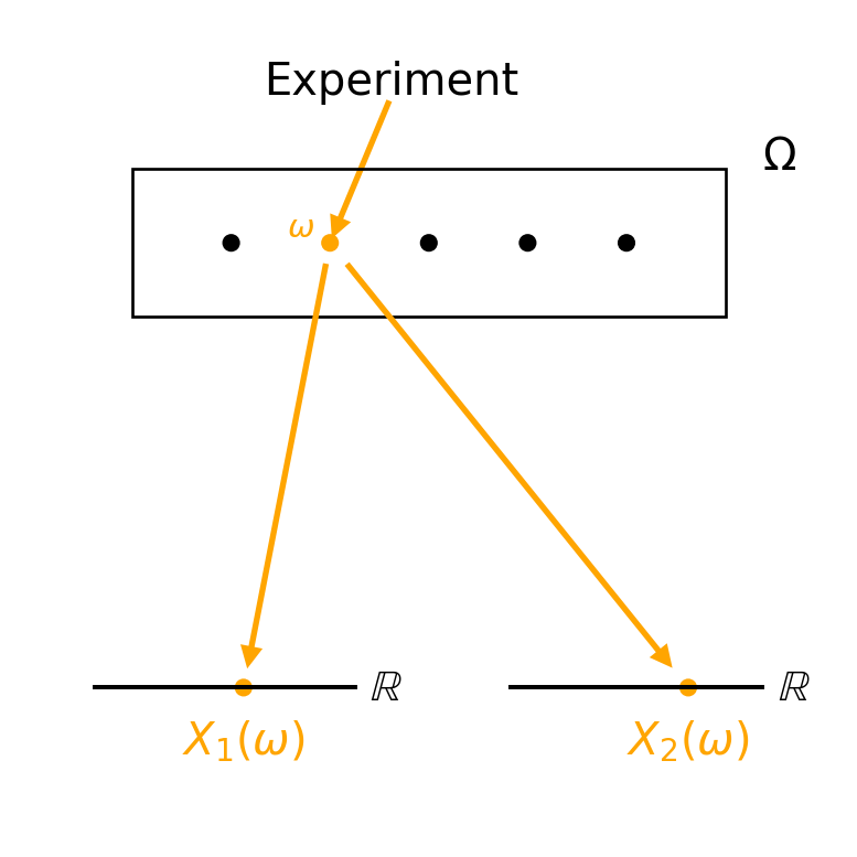
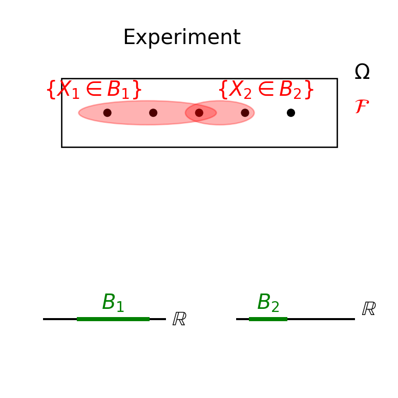
Mathematically it just means that we have multiple (measurable) functions, say $X_i: \Omega \to \R$, where we could have only finitely many (e.g. $i=1,\ldots,n$), countably infinite many (e.g. $i=1,2,\ldots$) or even uncountably many (we’ll encounter that situation in the context of stochastic process in continuous time later on in the course, we won’t consider it until that time). Visually, imagine that we extend the visuals in Figure 2.2 to contain (say) $n$ real lines rather than only one, and $n$ mappings say $X_1, \ldots, X_n$ that each map all $\omega \in \Omega$ to some value on their own real line. In Figure 2.2 (b) we would then see that the experiment is performed to obtain a certain outcome $\omega \in \Omega$, and plugging that into mappings they all take a value on their own real line. This creates a sequence of real numbers $X_1(\omega), X_2(\omega), \ldots, X_n(\omega) \in \R$.

Here is the key point, and the reason for writing a brief section about this: all of the stuff we have discussed in Section 2.3 and Section 2.5 applies (of course) to each $X_i$ individually. For any Borel set $B \in \mathcal{B}(\R)$, each $X_i$ has an inverse image $\{ X_i \in B\}=X_i^{-1}(B)$ which is some event in $\Omega$. Each $X_i$ has a distribution (as defined in Definition 2.5), a cdf, and is discrete, continuous or neither of these two. Etc.

But beyond that, we can now also look at events that involve two or more of the $X_i$’s. For instance, we could be interested in the event that $X_1$ is larger than $7$ and $X_2$ is less than $5$ (so, all outcomes in $\Omega$ for which both these inequalities hold) i.e. the event \[\{X_1>7 \text{ and } X_2<5\}=\{ \omega \in \Omega \, | \, X_1(\omega)>7 \text{ and } X_2(\omega)<5 \}.\] This is an example of an event that we can express in terms of inverse images of Borel sets, after all $\omega$ is an element of this event if and only it is an element of $\{X_1>7\}$ as well as of $\{X_2<5\}$, that is \[\{X_1>7 \text{ and } X_2<5\} = \{X_1>7\} \cap \{X_2<5\}.\] However it’s also easy to think of events that cannot be expressed using inverse images, for instance the event that $X_1$ is larger than $X_2$ i.e. \[\{X_1>X_2\}=\{ \omega \in \Omega \, | \, X_1(\omega)>X_2(\omega) \}.\]

Figure 2.3 visualises the case of two random variables.

(a) We have now two random variables, $X_1, X_2: \Omega \to \R$, who each map any $\omega \in \Omega$ to a value on their own real line. Then, when the experiment is executed and one of the possible outcomes, say $\omega$, is observed, they each take a value $X_1(\omega)$ and $X_2(\omega)$ on their real lines

Example 2.5 Consider the experiment of rolling two fair dice. Representing each outcome as a pair of numbers from $1$ to $6$ i.e. \[\begin{aligned} \Omega &= \{ \omega=(\omega_1,\omega_2) \, | \, \omega_1,\omega_2 \in \{1,\ldots,6\} \} \\ &= \{ (1,1), (1,2), \ldots, (1,6), (2,1), \ldots, (2,6), \ldots, (6,6)\} \end{aligned} \] there are 36 possible outcomes, all equally likely. This is again a “simple” experiment (cf. Example 2.2) and we can complete our probability space $(\Omega,\mathcal{F},\P)$ by setting $\mathcal{F}=\mathcal{P}(\Omega)$ and $\P$ is characterised by assigning probability $1/36$ to each outcome in $\Omega$.

We could for instance define the random variables $X_1$ and $X_2$ as the largest resp. smallest of the two numbers that we roll, i.e. $X_1, X_2: \Omega \to \R$ given by $X_1(\omega)=\max\{\omega_1,\omega_2\}$ and $X_2(\omega)=\min\{\omega_1,\omega_2\}$. Some examples of events are the following.

$\{X_1=6\}$ is an event containing $11$ outcomes: all pairs $(\omega_1,\omega_2)$ where $\omega_1=6$ or $\omega_2=6$ (or both).
$\{ X_2>4 \}=\{ (5,5), (5,6), (6,5), (6,6) \}$.
$\{ X_1=6 \text{ and } X_2>4 \}=\{ (5,6), (6,5), (6,6) \}$ — either directly or by using that this event is the intersection of $\{X_1=6\}$ and $\{ X_2>4 \}$.
$\{X_1=X_2\}=\{ (1,1), (2,2), \ldots, (6,6)\}$.
$\{X_1>X_2\}$ is an event containing $30$ outcomes (it is the complement of $\{X_1=X_2\}$).
$\{X_1<X_2\}=\emptyset$.

2.6.1 About independence

A final point that fits nicely here is to remind ourselves about independence. Recall that on some probablity space $(\Omega,\mathcal{F},\P)$, two events $A,B \in \mathcal{F}$ are called independent if it holds that $\P(A \cap B)=\P(A) \P(B)$ (don’t confuse this with disjoint i.e. $A \cap B=\emptyset$!).

Since $\sigma$-algebras are nothing but collections of events, this definition naturally extends: if $\mathcal{G}_1$ and $\mathcal{G}_2$ are two sub-$\sigma$-algebras of $\mathcal{F}$ then we call them independent if any two events $A \in \mathcal{G}_1$ and $B \in \mathcal{G}_2$ are independent i.e. if $\P(A \cap B)=\P(A) \P(B)$.

We can beautifully link this to our well known (from earlier probability courses) concept of independence of random variables. Recall from Definition 2.2 that any random variable $X$ i.e. $\mathcal{F}$-measurable function $X:\Omega \to \R$ comes with a generated $\sigma$-algebra $\sigma(X) \subseteq \mathcal{F}$. For any two such random variables $X, Y$, we can naturally define them to be independent if the $\sigma$-algebras $\sigma(X)$ and $\sigma(Y)$ to be independent. Keeping in mind that these generated $\sigma$-algebras consist of inverse images of Borel sets, this condition is equivalent to the condition that for any Borel sets $B_1, B_2 \in \mathcal{B}(\R)$ it holds that \[\P(X \in B_1 \text{ and } Y \in B_2)=\P(X \in B_1) \P(Y \in B_2).\] It can be shown that it is enough to consider only Borel sets of the form $(-\infty,x]$ (here is that magical collection from Section 1.6.2 again!) i.e. an equivalent condition is that \[\P(X \leq x \text{ and } Y \leq y)=\P(X \leq x) \P(Y \leq y) \quad \text{for all $x,y \in \R$.}\] This final formulation is the form you most likely encountered previously!

Exercises

You can now do Exercise 2.11.

2.7 Modes of convergence

As the final topic in this chapter we briefly look at the so-called modes of convergence (at least, the most commonly used ones). The setting is a probability space $(\Omega,\mathcal{F},\P)$ on which a sequence $X_1, X_2, \ldots$ of random variables is defined — in the vein of Section 2.6 our mental model is that each time we execute the experiment to observe an outcome $\omega \in \Omega$, they all take a value $X_1(\omega), X_2(\omega), \ldots \in \R$.

Now, whenever we have an infinite sequence of objects of some type, we can ask the question whether or not that sequence converges to some limit value (if it does, then the limit value is typically another object of the same type). Of course we all know quite well from our basic maths courses how this works for a sequence of numbers (if you’d like a reminder, see e.g. Wiki). However for more complicated objects you have to think about what “convergence” should exactly mean. It will always be a (context specific) interpretation of the general understanding we all have about “convergence”: the further along the sequence we travel, the smaller the distance between the element of the sequence and the limit value becomes, with that distance ultimately vanishing.

For a sequence of numbers $a_1, a_2, \ldots$ converging to a limit $a$, this general understanding easily and unambiguously translates to \[\lim_{n \to \infty} |a_n-a|=0. \tag{2.9}\] However for more complicated objects there is typically more than one way to measure distance and/or to interpret it vanishing, giving rise to multiple implementations of “convergence” — not (necessarily) competing with each other to be the “best” one but rather just creating multiple tools and to pick a suitable one from for the job at hand.

In the case of our sequence of random variables $X_1, X_2, \ldots$ on $(\Omega,\mathcal{F},\P)$, “convergence” should hence be to another random varable on $(\Omega,\mathcal{F},\P)$, say $X$. In line with the general understanding, we should look at the distances between $X_n$ and $X$ which naturally becomes \[Y_n = |X_n-X| \tag{2.10}\] (note that these $Y_n$’s are again random variables: $Y_n(\omega) = |X_n(\omega)-X(\omega)|$ for all $\omega \in \Omega$, cf. Proposition 2.1 for measurability). But then there are several different ways in which we could understand/define “$Y_n \to 0$ as $n \to \infty$”, leading to multiple different implementations/modes of convergence.

Remark 2.7. Note that a constant mapping i.e. for some $c \in \R$, $X(\omega)=c$ for all $\omega \in \Omega$, is always measurable (cf. Exercise 2.3 i) and hence always a random variable. You’ll sometimes encounter that we say that a sequence of random variables converges to some number, which is effectively just shorthand for saying that it converges to the corresponding constant random variable rather.

Here are the most common choices for defining “$Y_n \to 0$ as $n \to \infty$” i.e. possible modes of convergence.

Pointwise convergence: if for every $\omega \in \Omega$, the sequence $X_1(\omega), X_2(\omega), \ldots \in \R$ has a limit then we can define \[X(\omega):=\lim_{n \to \infty} X_n(\omega) \quad \text{for all $\omega \in \Omega$}.\] Then $X$ is a random variable (cf. Proposition 2.1 v) and we call $X$ the pointwise limit of the $X_n$’s.

Note, it is no problem for $X$ to take the values $-\infty$ and $\infty$ as well if needed (recall Remark 2.2 for our little cheat). Further, this mode only uses that the $X_n$’s are functions with a common domain, nothing (else) from the underlying probability space etc. Indeed this is just how pointwise convergence is defined for any old sequence of functions. It does not appear very often in Probability Theory.

Note that in Equation 2.10, this mode translates to $Y_n(\omega) \to 0$ for all $\omega \in \Omega$.
Almost sure convergence: this is a slightly weaker version of the previous one: the pointwise convergence from above is required to hold on any almost sure event (recall from Section 2.4) only, and we don’t care at all what happens on the complement of that event. That is to say, if $X$ is a random variable so that \[\P \left( \{ X=\lim_{n \to \infty} X_n \} \right) = \P \left( \{ \omega \in \Omega \, | \, X(\omega)=\lim_{n \to \infty} X_n(\omega) \} \right)=1 \tag{2.11}\] then we say that the $X_n$’s converge to $X$ almost surely, typically denoted “$X_n \stackrel{\text{a.s.}}{\longrightarrow} X$ as $n \to \infty$”.

Note that for Equation 2.11 to be able to hold, it must be the case that $\{ \lim_{n \to \infty} X_n \text{ exists}\}$ is an almost sure event (if it is not, then the $X_n$’s simply do not have an almost sure limit). If this is the case, then setting e.g. \[X(\omega)=\begin{cases} \lim_{n \to \infty} X_n(\omega) & \text{if the limit exists} \\ 0 & \text{otherwise} \end{cases} \] gives a random variable (Proposition 2.1 v) for which Equation 2.11 holds i.e. to which the $X_n$’s converge almost surely (as above, we allow the values $-\infty$ and $\infty$ again as well). But it is not the only possible choice we could make, for one reason because the choice for the value $0$ in the “otherwise” case is arbitrary.

Indeed in the case of almost sure convergence, the limit is not uniquely defined (all a consequence of not caring about what happens outside an almost sure event): if there is a random variable that is an almost sure limit value, then there are many others that are equally valid limit values as well! This may seem strange at first, but as you gain more experience you’ll realise that actually it is quite natural since a lot of the time, we work on almost sure basis only anyway, and on that basis all the possible limiting values are effectively the same (see also Exercise 2.13).

Note that in Equation 2.10, this mode translates to: there exists an almost sure event so that $Y_n(\omega) \to 0$ for all $\omega$ in that event.
Convergence in probability: if a random variable $X$ exists so that \[\text{for any $\eps>0$:} \quad \lim_{n \to \infty} \P(|X_n-X|>\eps)=0\] then we say that the $X_n$’s converge to $X$ in probability, typically denoted “$X_n \stackrel{\P}{\longrightarrow} X$ as $n \to \infty$”.

As in the case of almost sure convergence, the limit $X$ is not uniquely defined (may vary on the complement of an almost sure event). Note that the link with Equation 2.10 is obvious now.
Convergence in r-th mean/in $L^r$ (for some $r \geq 1$): if a random variable $X$ exists so that \[\lim_{n \to \infty} \E \left[ |X_n-X|^r \right] =0 \tag{2.12}\] then we say that the $X_n$’s converge to $X$ in $r$-th mean or in $L^r$, typically denoted “$X_n \stackrel{L^r}{\longrightarrow} X$ as $n \to \infty$”.

Again the limit $X$ may vary on the complement of an almost sure event, and the link with Equation 2.10 is again obvious. Note that there is one problem: Equation 2.12 involves an expectation, and currently we only have these defined for the special cases of discrete and continuous random variables (recall from Section 2.5.1). However in the next chapter we’ll develop an understanding of expectation that works for any random variable and then this mode of convergence is properly defined for all random variables as well! As we will see in that chapter, in general the expectation of a random variable can be expressed as an integral (of a new, to be defined type!). That will put us in the context of $L^r$ spaces and explains the at this point slightly mysterious “in $L^r$” terminology, cf. Remark 3.3.
Convergence in distribution: this is an odd one out in the sense that it is not some interpretation of the $Y_n$’s (from Equation 2.10) vanishing. Rather it focuses on the distributions (cf. Definition 2.5) of the random variables involved. Basically we want to express the circumstance that the distributions $\mu_{X_n}$ of the $X_n$’s converge to the distribution $\mu_X$ of some random variable $X$. This is easiest expressed in terms of cdf’s (cf. Definition 2.6): we say that the $X_n$’s (with cdf’s $F_{X_n}$’s) converge in distribution to (the distribution of) $X$ (with cdf $F_X$) if it holds that
\[\lim_{n \to \infty} F_{X_n}(x)=F(x) \quad \text{for all $x \in \R$ in which $F$ is continuous.}\]

There is not really a standard notation for this one (numerous different ones are generally used) so let’s simply not have one. Obviously, all that matters about the limit is its distribution, and therefore sometimes you also see a statement where only the limit distribution is mentioned, e.g. like “$X_n$ converges in distribution to $\mathcal{N}(0,1)$”.

A consequence of focussing on distrbutions only is that the random variables involved do not even need to be defined on the same probability space!

Of course, there is a lot more to say here — for instance: can we specify relatively easy to verify conditions that imply any of these modes of convergence, and how do they interact with each other i.e. does one mode of convergence imply the other, etc. Unfortunately we don’t have scope/time to address such questions (though some of it we’ll see back in the next chapter). If you’re interested in a nice exploration, see e.g. Section 7.2 in Grimmett and Stirzaker (1992).

Exercises

You can now do Exercise 2.12–Exercise 2.13.

2.8 Some exercises

About the exercises

Each exercise has a (rough) indication of its difficulty, as follows:

*	easier: can be solved by (almost) only using relevant definitions/results,
**	medium: in addition to relevant definitions/results, needs a limited amount of work/creativity,
*******	harder: in addition to relevant definitions/results, needs a larger amount of work/serious creativity,
💀	warning: might make your brain hurt! These are mainly intended to provide some extra challenge for those of you keen on that and are generally quite hard. You don't need to worry about these too much for exam purposes.

The exam consists of mostly ** and *** level questions, some *, and possibly at most a few marks worth of 💀.

A bit of preaching: it is an incredibly important part of the study process to try and work on the exercises as much as possible. To become a better mathematician/learn new maths (and also to get a good exam mark ;)), above all you need to do it. And yes, of course that includes falling over things, and making mistakes, and getting stuck, and getting frustrated — all part of the game and what you’re supposed to be doing! Your lecturers have done that as well and still do it. What matters is that you don’t let that discourage you and that you make good use of the help and resources available to help you develop your skills. As part of that, many exercises have a hint in a block like this:

Hint (click to view)

Hint!

These are trying to help you on your way if you don’t know where to start or to provide some ideas if you get stuck. In spirit of the above, always have a look at these first and try again before you look at the full solution. (These hints are an extra service that won’t be available in the exam I’m afraid ;).)

Of course, we have our classes and there’s office hours, email etc. as well — I’m at any time very happy to help you with any questions you may have, and you should please never feel that any question is “too dumb” to ask!

Full/detailed solutions for the exercises will become available, just immediately below the exercises, after our Friday tutorial.

Exercise 2.1 [*/**] Prove Lemma 2.1.

Bonus: if we would formulate Lemma 2.1 ii with images rather than inverse images, then it would read “if $A_1, A_2, \ldots$ is a partition of $E$, then $f(A_1), f(A_2), \ldots$ is a partition of $G$”. Can you explain why this statement is not generally true?

Hint (click to view)

All you need is the definition of inverse images. For Lemma 2.1 ii, to prove the mutually disjoint property, you could argue by contradiction i.e. assume that they are not mutually disjoint and work towards a consequence that we know to be false.

Full solution (click to view)

For Lemma 2.1 i, let’s do the statement that \[f^{-1} \left( \bigcup_{i=1}^\infty B_i \right) = \bigcup_{i=1}^\infty f^{-1}(B_i).\] We could e.g. use the “show both inclusions” strategy (cf. Remark 1.1 iii). If $x$ is an element of the left hand side, then by def of the inverse image we get that $f(x) \in \cup_{i=1}^\infty B_i$ and hence there is a $j \geq 1$ so that $f(x) \in B_j$. But then, again by def of the inverse image, it follows that $x \in f^{-1}(B_j)$ and hence $x$ is also in the union of the $f^{-1}(B_i)$’s i.e. of the right hand side. To argue the other inclusion, you can just use this argument again the other way around (all steps are actually “if and only if”).

For Lemma 2.1 ii, following Section 1.2.3, we need to show two points: that the collection of subsets $f^{-1}(B_1), f^{-1}(B_2), \ldots$ covers the whole of $E$, and that they are mutually disjoint.

For the first point, pick any $x \in E$. Our function $f$ maps it to some value $f(x) \in G$. Since $B_1, B_2, \ldots$ covers the whole of $G$, $f(x)$ must be in $B_j$ for some $j \geq 1$. But then, by definition, $x \in f^{-1}(B_j)$. So indeed $x \in \cup_{i=1}^\infty f^{-1}(B_i)$.

For the second point, assume that they are not mutually disjoint i.e. that some $i$ and $j$ exist so that $f^{-1}(B_i) \cap f^{-1}(B_j) \not= \emptyset$. Pick some $x \in f^{-1}(B_i) \cap f^{-1}(B_j)$. The fact that $x \in f^{-1}(B_i)$ means (by def) that $f(x) \in B_i$. In the same way it follows that $f(x) \in B_j$ i.e. $f(x) \in B_i \cap B_j$. But this is impossible, since $B_1, B_2, \ldots$ are mutually disjoint we know that $B_i \cap B_j=\emptyset$, so we have arrived at a contradiction.

Finally for the bonus: this statement fails for instance if $f$ is not “onto”/surjective, that is if there is some $y \in G$ that is never visited by $f$ i.e. if for all $x \in G$ it holds that $f(x) \not= y$, because then $y$ is not an element of any of the $f(A_i)$’s and hence the $f(A_i)$’s do not cover the whole of $E$. It can also fail if $f$ is “many-to-one”/not injective i.e. if $x_1 \not= x_2 \in E$ exist so that $f(x_1)=f(x_2)$. If $x_1 \in A_i$ and $x_2 \in A_j$ for $i \not= j$, then $y \in f(A_i) \cap f(A_j)$ i.e. the $f(A_i)$’s are not mutually disjoint. Indeed the bonus statement is only guaranteed to hold if $f$ is a bijection!

Exercise 2.2 [*] Let $(E,\mathcal{F})$ be a measurable space and $f: E \to \R$ a measurable function. Explain why it must be true that $\sigma(f)$ is a sub-$\sigma$-algebra of $\mathcal{F}$ i.e. $\sigma(f) \subseteq \mathcal{F}$.

Full solution (click to view)

Recall the collection of subsets of $E$ that we used in Definition 2.2: \[\mathcal{C}=\{ f^{-1}(B) \, | \, B \in \mathcal{B}(\R) \}.\] From Definition 2.1 we know that each element in $\mathcal{C}$ is also an element of $\mathcal{F}$. But from Definition 1.2 we know that $\sigma(f)=\sigma(\mathcal{C})$ is the smallest $\sigma$-algebra containing these elements i.e. that $\sigma(f) \subseteq \mathcal{F}$.

Exercise 2.3 [**] Let $(E,\mathcal{F})$ be a measurable space. Below we define three functions, show that all of them are measurable.

Fix some $y \in \R$, and consider the constant function $f: E \to \R$ given by $f(x)=y$ for all $x \in \R$.
Fix any $A \in \mathcal{F}$. We define the indicator function of $A$ as the function⁹ $\mathbf{1}_A: E \to \R$ given by \[ \mathbf{1}_A(x)=\begin{cases} 1 & \text{if $x \in A$} \\ 0 & \text{if $x \not\in A$.} \end{cases} \]
Suppose that $A_1, \ldots, A_n \in \mathcal{F}$ form a partition (cf. Section 1.2.3) of $E$, and fix values $y_1, \ldots, y_n \in \R$. Let $f: E \to \R$ be the function given by $f(x)=y_i$ if $x \in A_i$.

⁹ Because indicator functions are such fundamental building blocks (as we’ll see later) we use the special symbol “$\mathbf{1}_A$” rather than a more generic “$f$” (or whatever else)

Hint (click to view)

For i and ii, all you need is either Definition 2.1 or Proposition 2.1 i (whichever you prefer). For iii, find a way to express $f$ as a linear combination of indicator functions — if you manage to do that you can make use of ii and are quickly done!

Full solution (click to view)

You can argue either directly from Definition 2.1 (because this $f$ is so straightforward) or use Proposition 2.1 i for instance. Going with the former, the key point to realise is that since any $x \in E$ gets mapped to $y$, for any Borel set $B$ we either have $f^{-1}(B)=E$ (if $y \in B$) or $f^{-1}(B)=\emptyset$ (if $y \not\in B$). So $f$ is measurable if both $E$ and $\emptyset$ are elements of $\mathcal{F}$, and this holds for any $\sigma$-algebra (cf. Definition 1.1 and Exercise 1.1).
Similar as for i, you can use either Definition 2.1 or Proposition 2.1 i. Let’s now go with the latter one. Keeping in mind that each $x \in E$ gets mapped to either $0$ or $1$, we have the following three cases: if $a<0$ then $f^{-1}((-\infty,a])=\emptyset$, if $a \in [0,1)$ then $f^{-1}((-\infty,a])=A^c$, and if $a \geq 1$ then $f^{-1}((-\infty,a])=E$. As already argued in i above, we know that $\emptyset$ and $E$ are elements of any $\sigma$-algebra, and so is $A^c$ since we assumed that $A$ is (cf. Definition 1.1 ii).
We could use the same approach as in i and ii, but there is also a shorter route (which will come in handy later as well!). The key is to consider the indicator functions $\mathbf{1}_{A_1}, \mathbf{1}_{A_2}, \ldots, \mathbf{1}_{A_n}$. Note that for any $x \in E$, since $A_1, \ldots, A_n$ form a partition of $E$, it holds that exactly one of the numbers $\mathbf{1}_{A_1}(x), \mathbf{1}_{A_2}(x), \ldots, \mathbf{1}_{A_n}(x)$ equals $1$ (and hence the others all equal $0$). This means that we can express $f$ in the following way: \[f(x)=\sum_{j=1}^n y_j \mathbf{1}_{A_j}(x) \quad \text{for all $x \in E$}. \tag{2.13}\] To write out the argument in detail: take any $x \in E$. Then there exists $i \in \{1,\ldots,n\}$ so that $x \in A_i$ and $x \not\in A_j$ for $j \not= i$. Hence $\mathbf{1}_{A_i}(x)=1$ and $\mathbf{1}_{A_j}(x)=0$ for all $j \not= i$, which gives indeed \[\sum_{j=1}^n y_j \mathbf{1}_{A_j}(x) = y_i \cdot 1 = y_i = f(x).\] And here is the reason why Equation 2.13 is so helpful: it shows that we can write $f$ as a linear combination of indicator functions. We know from ii above (and because we assumed that the $A_i$’s are measurable sets) that each of these indicator functions is measurable. And then it follows immediately from Proposition 2.1 iv that $f$ is measurable as well.

Exercise 2.4 [*] Let $(\Omega,\mathcal{F},\P)$ be a probability space. Show that an event $A \not= \Omega$ exists with $\P(A)=1$ if and only if an event $N \not= \emptyset$ exists with $\P(N)=0$.

Full solution (click to view)

Recall that a general strategy for proving that two statements are equivalent is to show that the first implies the second as well as that the second implies the first.

Given an event $A \not= \Omega$ with $\P(A)=1$, we can choose $N=A^c$: this is also an event (cf. Definition 1.1 ii), it is not the empty set since $A \not= \Omega$, and $\P(A^c)=1-\P(A)=0$ (this rule we all know quite well we haven’t yet encountered in this particular form, but it follows for instance from countable additivity, cf. Definition 1.3 ii: since $A \cup A^c=\Omega$, $\P(A)+\P(A^c)=\P(\Omega)=1$). You go the other way!

Exercise 2.5 [**] Suppose that $A_1, A_2, \ldots$ is a sequence of almost sure events on some probability space. Why is it clear that for any $n \geq 1$, $\bigcup_{i=1}^n A_i$ is an almost sure event as well? Show that also $\bigcap_{i=1}^\infty A_i$ is an almost sure event.

Hint (click to view)

For the second one, looking through the properties of (probability) measures in Section 1.5 we don’t really have anything to deal with an intersection but we do have some to deal with unions. How do we relate unions and intersections again? Well we have the De Morgan’s laws (cf. Remark 1.1) e.g.!

Full solution (click to view)

For the first one, basically the idea is that by taking unions sets can only grow, not shrink, and hence their probablity measure can only get larger as well. Specifically, you could for instance use that since $A_1 \subseteq \bigcup_{i=1}^n A_i$, we get from Theorem 1.1 i that \[1=\mu(A_1) \leq \mu \left( \bigcup_{i=1}^n A_i \right).\]

For the second one, from De Morgan’s laws (cf. Remark 1.1) we know that \[\left( \bigcap_{i=1}^\infty A_i \right)^c = \bigcup_{i=1}^\infty A_i^c.\] Since the $A_i$’s are almost sure events, $\P(A_i^c)=1-\P(A_i)=0$ and by subadditivity (cf. Theorem 1.1 iii) \[\P \left( \bigcup_{i=1}^\infty A_i^c \right) \leq \sum_{i=0}^\infty \P(A_i^c)=0.\] So indeed \[\P \left( \bigcap_{i=1}^\infty A_i \right)=1- \P \left( \left( \bigcap_{i=1}^\infty A_i \right)^c \right) \geq 1-0=1.\]

Exercise 2.6 [*/**] Let $(\Omega,\mathcal{F},\P)$ be a probability space on which a random variable $X: \Omega \to \R$ lives. Show that the mapping $\mu_X: \mathcal{B}(\R) \to [0,1]$ given by Equation 2.3 is indeed a probability measure on $(\R,\mathcal{B}(\R))$.

Hint (click to view)

Note that the job is to verify that $\mu_X$ satisfies the conditions of Definition 1.3, where $(E,\mathcal{F})=(\R,\mathcal{B}(\R))$. The definition of $\mu_X$ means that you need to work with inverse images under $X$, for this recall the general properties of inverse images we have seen in Section 2.2 and the work we have done in Exercise 2.1!

Full solution (click to view)

We need to verify that $\mu_X$ satisfies the conditions of Definition 1.3, where $(E,\mathcal{F})=(\R,\mathcal{B}(\R))$ obviously:

Since the event $\{ X \in \emptyset \}=X^{-1}(\emptyset)=\emptyset$ (recall from the convention mentioned in Section 2.2), we get that \[\mu_X(\emptyset)=\P(X \in \emptyset)=\P(\emptyset)=0,\] the final equality because $\P$ is a probability measure i.e. satisfies the conditions in Section 2.2.
for mutually disjoint Borel sets $B_1, B_2, \ldots$ we get from Lemma 2.1 i that \[X^{-1} \left( \bigcup_{i=1}^\infty B_i \right) = \bigcup_{i=1}^\infty X^{-1}(B_i),\] and hence \[\begin{aligned} \mu_X \left( \bigcup_{i=1}^\infty B_i \right) &= \P \left( X^{-1} \left( \bigcup_{i=1}^\infty B_i \right) \right) \\ &= \P \left( \bigcup_{i=1}^\infty X^{-1}(B_i) \right) = \sum_{i=1}^\infty \P(X^{-1}(B_i))= \sum_{i=1}^\infty \mu_X(B_i), \end{aligned} \] where the third equality uses that the events $X^{-1}(B_1), X^{-1}(B_2), \ldots$ are mutually disjoint because the $B_i$’s are mutually disjoint (this follows from the same arguments used to prove Lemma 2.1 ii, see also Exercise 2.1 above), and that $\P$ is a (probablity) measure.

So now we know that $\mu_X$ is indeed a measure, to conclude that it is in particular a probability measure note that $\mu_X(\R)=\P(X^{-1}(\R))=\P(\Omega)=1$ since $\P$ is a probability measure.

Exercise 2.7 [**] Fix some probability measure $\mu$ on $(\R,\mathcal{B}(\R))$. Construct a probablity space $(\Omega,\mathcal{F},\P)$ with random variable $X: \Omega \to \R$ so that $X$ has distribution $\mu$.

Hint (click to view)

The hint is that you don’t at all need a hint, because the solution is a one liner! Really!

Full solution (click to view)

Take $\Omega=\R$, $\mathcal{F}=\mathcal{B}(\R)$ and $\P=\mu$, and let $X: \Omega \to \R$ be the identity mapping i.e. $X(\omega)=\omega$ for all $\omega \in \Omega=\R$. Then, following Definition 2.5, with $\mu_X$ denoting the distribution of $X$, we get for any Borel set $B$ that \[\mu_X(B)=\P(X \in B)=\P(B)=\mu(B)\] (the second equality uses that since $X$ is the identity mapping, the event $\{X \in B\}$ is just equal to the event $B$). So indeed $\mu_X=\mu$ and we’re done. I know!

Exercise 2.8 [*/**] Consider again experiment 1 in Example 2.3: the experiment of flipping a coin with a random variable $X$ that takes the value $0$ if tails and $1$ if heads. Suppose that we allow the coin to be unfair i.e. we replace the probability measure $\P_1$ in the example with the one specified on the singletons as follows: \[\Q_\alpha(\{T\})=\alpha \quad \text{and} \quad \Q_\alpha(\{H\})=1-\alpha,\] where $\alpha \in (0,1)$ is a parameter.

What is now the distribution $\mu_X$ of $X$? Do you recognise it as one of the “famous” ones with its own name?

Note: part of the goal of this execise is to stress the point also made in Section 2.3, which is rather obvious in that section but people sometimes tend to forget as they march on: the distribution of a random variable (also) depends on the probability measure used!

Full solution (click to view)

Note that much of the work we already did in Example 2.3 remains the same, in particular since $X$ still takes the values $0$ or $1$, for any Borel set $B$ we still need to consider the same cases (i.e. whether $B$ contains $0$ or $1$ or neither or both), except now with probabilities \[\Q_\alpha(X=0)=\alpha \quad \text{and} \quad \Q_\alpha(X=1)=1-\alpha.\] This brings us to \[\mu_{X}(B)=\begin{cases} 0 & \text{if $0 \not\in B$ and $1 \not\in B$} \\ \alpha & \text{if $0 \in B$ and $1 \not\in B$} \\ 1-\alpha & \text{if $0 \not\in B$ and $1 \in B$} \\ 1 & \text{if $0 \in B$ and $1 \in B$.} \end{cases} \] Since $X$ takes the values $0$ and $1$ with probabilities $\alpha$ and $1-\alpha$, it is (still) a Bernoulli distribution but now with parameter $1-\alpha$!

Exercise 2.9 [**/***] On a probablity space $(\Omega,\mathcal{F},\P)$, let $X$ and $Y$ be two random variables that are equal almost surely. Show that $X$ and $Y$ have the same distribution.

Hint (click to view)

Make sure that you read “are equal almost surely” correctly: “are equal” simply means that they are the same mappings, i.e. that $X(\omega)=Y(\omega)$ for all $\omega \in \Omega$. The qualifier “almost surely” means, as discussed in Section 2.4, that this property is not necessarily true on the whole of $\Omega$ but it holds that the event $\{X=Y\}=\{ \omega \in \Omega \, | \, X(\omega)=Y(\omega) \}$ has probability $1$. Further, if you’re not sure where to start, then consider the inverse image of any $B$ as consisting of two parts: the part inside the event $\{X=Y\}$ and the part outside of it.

Full solution (click to view)

Following Definition 2.5, we need to show that $\mu_X=\mu_Y$ i.e. that for any Borel set $B$ we have that $\P(X \in B)=\P(Y \in B)$. The trick is to consider the inverse image of any Borel set $B$ as consisting of two parts: the part inside the event $A:=\{X=Y\}$ and the part outside of it, that is \[\{X \in B\}=(\{X \in B\} \cap A) \cup (\{X \in B\} \cap A^c)\] and \[\{Y \in B\}=(\{Y \in B\} \cap A) \cup (\{Y \in B\} \cap A^c).\] Starting with the first one, note that this is a union of disjoint events and hence by countable additivity (cf. Definition 1.3) \[\P(X \in B)=\P(\{X \in B\} \cap A) + \P(\{X \in B\} \cap A^c).\] Note that since $\P(A)=1$ we know that $\P(A^c)=1-\P(A)=0$ (see also Exercise 2.4). Since $\{X \in B\} \cap A^c$ is a subset of $A^c$ it follows from Theorem 1.1 i that $\P(\{X \in B\} \cap A^c)=0$. So we can simplify to (the same argument applies to $Y$) \[\P(X \in B)=\P(\{X \in B\} \cap A) \quad \text{and} \quad \P(Y \in B)=\P(\{Y \in B\} \cap A). \tag{2.14}\] Finally, note that $\{X \in B\} \cap A=\{Y \in B\} \cap A$, since the intersection with $A$ guarantees that any $\omega$ that is an element of the left or right hand side has the property that $X(\omega)=Y(\omega)$. So these events have the same probability and using Equation 2.14 we indeed arrive at \[\P(X \in B)=\P(\{X \in B\} \cap A)=\P(\{Y \in B\} \cap A)=\P(Y \in B).\]

Exercise 2.10 [*/**] Let $X$ be a continous random variable on some probability space. Show that for any $x \in \R$, we have that $\P(X=x)=0$.

Note: on the one hand, as we know well by now, each time we execute the experiment, $X$ takes a value somewhere on the real line. Yet on the other hand, this execise shows that if you fix any point on the real line and ask “What is the probability that $X$ ends up in that fixed point?” then the answer is “$0$”. That is counterintuitive, yet it is just again our intuition failing in the face of the Uncountability Dragons, in this case because the set of points where $X$ can end up, i.e. its range, is uncountable!

Hint (click to view)

If you’re not sure where to start, then think of a way to capture $x$ in a small interval and express the probability of $X$ ending up in that interval using its cdf.

Full solution (click to view)

There is several ways to do this, but either way, the only thing we know about continuous random variables that is specific for them is the info about its cdf from Section 2.5.1 so we’ll want to use that somehow. For the given $x \in \R$ we could for instance say that for any $n=1,2,\ldots$, $\{x\} \subseteq (x-1/n,x]$ and hence by Theorem 1.1 i (twice) and the def of the cdf \[\begin{aligned} & \P(X=x) \leq \P(X \in (x-1/n,x]) = \P(X \in (-\infty,x] \setminus (-\infty,x-1/n]) \\ & = \P(X \in (-\infty,x])-\P(X \in (-\infty,x-1/n])=F_X(x)-F_X(x-1/n). \end{aligned} \] Since $F_X$ is a continuous function (as we know from Section 2.5.1), we have that $F_X(x-1/n) \to F_X(x)$ as $n \to \infty$ and hence it follows that indeed $\P(X=x)=0$.

Note: recall from Definition 2.6 that a general cdf is only guaranteed to be right-continuous, not necessarily left-continuous (everywhere). Since $x-1/n \uparrow x$ as $n \to \infty$, the above argument would fail to hold if $F_X$ was not left-continuous in $x$. So indeed for random variables that are not continuous and hence do not necessarily have a (left-)continuous cdf, the statement in this exercise is not necessarily true!

Exercise 2.11 [**] On some probablity space $(\Omega,\mathcal{F},\P)$, consider two events $A_1, A_2 \in \mathcal{F}$. Recall from Exercise 2.3 that any event naturally comes with a measurable indicator function which is hence also a random variable, which in turns naturally comes with a generated $\sigma$-algebra (cf. Definition 2.2). Let $\mathbf{1}_{A_1}$ and $\mathbf{1}_{A_2}$ be the indicator function of $A_1$ and $A_2$. Show that the following statements are equivalent:

$A_1$ and $A_2$ are independent events,
$\sigma(\mathbf{1}_{A_1})$ and $\sigma(\mathbf{1}_{A_2})$ are independent $\sigma$-algebras.

Note: recall from Section 2.6.1 that statement ii is equivalent to/can be taken as the definition of $\mathbf{1}_{A_1}$ and $\mathbf{1}_{A_2}$ being independent random variables.

Hint (click to view)

This should be pretty straightforward from the discussion of independence in Section 2.6.1, after you’ve worked out what $\sigma(\mathbf{1}_{A_1})$ and $\sigma(\mathbf{1}_{A_2})$ are (for which you maybe want to look back at your solution of Exercise 2.3).

Further, in general a strategy for proving that two statements are equivalent is to show that each implies the other. For i implies ii you “just” need to work out all possible event pairs!

Full solution (click to view)

Let’s first work out what these $\sigma$-algebras exactly are, following Definition 2.2. Note that, partly using the same arguments as in Exercise 2.3, since for any $A \in \mathcal{F}$ $\mathbf{1}_A$ maps $\omega \in A$ to $1$ and $\omega \in A^c$ to $0$, for any Borel set $B \in \mathcal{B}(\R)$ we have that $\mathbf{1}_A^{-1}(B)$ is one of $\emptyset$ (if $0 \not\in B$ and $1 \not\in B$), $A$ (if $0 \not\in B$ and $1 \in B$), $A^c$ (if $0 \in B$ and $1 \not\in B$) or $\Omega$ (if $0 \in B$ and $1 \in B$). So we see that \[\sigma(\mathbf{1}_{A_1})=\left\{ \emptyset, A_1, A_1^c, \Omega \right\} \quad \text{and} \quad \sigma(\mathbf{1}_{A_2})=\left\{ \emptyset, A_2, A_2^c, \Omega \right\}.\]

Now on to proving that both statements are indeed equivalent.

For ii implies i, that’s nice and easy because by def (cf. Section 2.6.1), if $\sigma(\mathbf{1}_{A_1})$ and $\sigma(\mathbf{1}_{A_2})$ are independent then any pair of events, one from the first and one from the second, is independent. So we can simply apply this with $A_1$ from $\sigma(\mathbf{1}_{A_1})$ and $A_2$ from $\sigma(\mathbf{1}_{A_2})$.

For i implies ii, assuming that $A_1$ and $A_2$ are independent we need to show that any pair of events, one from $\sigma(\mathbf{1}_{A_1})$ and one $\sigma(\mathbf{1}_{A_2})$, let’s denote them by $C_1$ and $C_2$, are also independent. For this, note that the equality \[\P(C_1 \cap C_2)=\P(C_1) \P(C_2)\] is trivially true if $C_1=\Omega$ (then both sides equal $\P(C_2)$) and if $C_1=\emptyset$ (then both sides equal $0$). By symmetry of course the same holds if $C_2=\Omega$ or $C_2=\emptyset$. By assumption it also holds if $C_1=A_1$ and $C_1=A_1^c$.

Now suppose that $C_1=A_1^c$ and $C_2=A_2$, i.e. we need to work out $\P(A_1^c \cap A_2)$. We do know what $\P(A_1 \cap A_2)$ is, we need to make the step to $A_1^c$. The obvious link between $A_1$ and $A_1^c$ is that they form a partition of $\Omega$ so we’ll need to use that to bridge the gap. One way to do that is as follows: \[\begin{aligned} \P(A_2) &= \P(\Omega \cap A_2) \\ &= \P((A_1 \cup A_1^c) \cap A_2) \\ &= \P((A_1 \cap A_2) \cup (A_1^c \cap A_2)) \\ &= \P(A_1) \P(A_2) + \P(A_1^c \cap A_2) \end{aligned} \] (where the third equality uses distributivity on Wiki, the fourth uses countable additivity (cf. Definition 1.3) — indeed these sets are disjoint as one is contained in $A_1$ and the other in $A_1^c$ — plus independence of $A_1$ and $A_2$) and hence indeed \[\P(A_1^c \cap A_2)=\P(A_2) (1-\P(A_1))=\P(A_2) \P(A_1^c).\]

Finally, you can deal with the remaining case in the same way (in fact, it is obvious that this is the case by symmetry).

Exercise 2.12 [*/**] On the probability space $([0,1],\mathcal{B}([0,1]),\lambda)$, where $\lambda$ is the Lebesgue measure (i.e. the same probability space as we used in Example 2.2 iv), consider the sequence of random variables $X_1, X_2, \ldots$ given by, for all $n \geq 1$ \[X_n(\omega)=\begin{cases} 1/n & \text{if $\omega \in [0,1/2)$} \\ 0 & \text{if $\omega \in [1/2,1]$.} \end{cases} \] Are the $X_n$’s discrete, continuous, or “other” random variables?

Under each of the following modes of convergence: almost surely, in probability and in $L^r$ (for $r \geq 1$), investigate whether the sequence has a limit. If so, give a limit and prove that you’re correct.

Full solution (click to view)

Since each $X_n$ takes only two possible values ($1/n$ and $0$), they are all discrete (cf. Section 2.5.1). Further, since $1/n \to 0$ as $n \to \infty$, we have that $X_n$ converges pointwise to the constant random variable $X(\omega)=0$ for all $\omega \in \Omega$, and we could guess that this is a limit under each of the three requested modes of convergence as well.

For almost sure convergence, we already discussed that $X_n(\omega) \to X(\omega)$ as $n \to \infty$ for all $\omega \in \Omega$, so the pointwise convergence holds even on the whole $\Omega$ which is trivially an almost sure event.
For convergence in probability, fix any $\eps>0$. For any $\omega \in \Omega$, since $X=0$ and $X_n$ is non-negative, $|X_n(\omega)-X(\omega)|=X_n(\omega)$. Looking at the event we are interested in, we see that \[\{ |X_n-X|>\eps \}=\{X_n>\eps\}=\begin{cases} [0,1/2) & \text{if $n<1/\eps$} \\ \emptyset & \text{if $n \geq 1/\eps$.} \end{cases} \] So in particular for all $n \geq 1/\eps$ \[\P(|X_n-X|>\eps)=\P(\emptyset)=0,\] proving that indeed $\lim_{n \to \infty} \P(|X_n-X|>\eps)=0$.
Finally for convergence in $L^r$, defining the random variables $Y_n := |X_n-X|^r$ we can work these out as \[Y_n(\omega)=\begin{cases} 1/n^r & \text{if $\omega \in [0,1/2)$} \\ 0 & \text{if $\omega \in [1/2,1]$.} \end{cases} \] Since the $Y_n$’s are discrete random variables, we can work out their expectation using Equation 2.6 (with $h$ just the identity function) \[\E[Y_n]=\frac{1}{n^r} \P(Y_n=1/n^r)+0=\frac{1}{n^r} \lambda([0,1/2))=\frac{1}{2 n^r}\] which indeed vanishes as $n \to \infty$. (Of course, if you prefer you could equivalently also use Equation 2.6 directly on $|X_n-X|^r$ by seeing this expression as $h(X_n)$ etc.).

Exercise 2.13 [**] On some probability space $(\Omega,\mathcal{F},\P)$, let $X, Y, X_1, X_2, \ldots$ all be random variables and suppose that $X_n \stackrel{\text{a.s.}}{\longrightarrow} X$ as $n \to \infty$. Show that $X_n \stackrel{\text{a.s.}}{\longrightarrow} Y$ as $n \to \infty$ holds if and only if $X=Y$ a.s.

Hint (click to view)

Consider the three events $A=\{X_n \to X\}$, $B=\{X_n \to Y\}$ and $C=\{X=Y\}$, how do these relate to each other? Exercise 2.5 may come in handy as well.

Full solution (click to view)

Define the three events $A=\{X_n \to X\}$, $B=\{X_n \to Y\}$ and $C=\{X=Y\}$ (write them out in their full/longhand versions — cf. Section 2.3 — if that makes it easier for you to see what is going on!). Then we know that $A$ is an almost sure event.

Recall that to show an equivalence i.e. an “if and only if”, one generally good strategy is to prove both implications.

First assume that $X_n \stackrel{\text{a.s.}}{\longrightarrow} Y$ as $n \to \infty$ i.e. that $B$ is also an almost sure event. Now suppose that $\omega \in \Omega$ is such that $X_n(\omega) \to X(\omega)$ and $X_n(\omega) \to Y(\omega)$ (i.e. $\omega \in A \cap B$). Then it immediately follows that also $X(\omega)=Y(\omega)$ i.e. that $\omega \in C$. This means that we have $A \cap B \subseteq C$. Since $A$ and $B$ are alomost sure events, we get from Exercise 2.5 that also $A \cap B$ is an almost sure event. Since $A \cap B \subseteq C$, also $C$ is an almost sure event (using e.g. Theorem 1.1 i).

Now assume that $X=Y$ a.s. i.e. that $C$ is an almost sure event. Very similar to above we can derive that $A \cap C \subseteq B$ and that hence $B$ is an almost sure event as well.