\[ \renewcommand{\P}{\mathop{\mathbb{P}}\nolimits} \newcommand{\E}{\mathop{\mathbb{E}}\nolimits} \newcommand{\var}{\mathop{\rm Var}\nolimits} \newcommand{\cov}{\mathop{\rm Cov}\nolimits} \newcommand{\limsup}{\mathop{\rm limsup}} \newcommand{\liminf}{\mathop{\rm liminf}} \newcommand{\R}{\mathbb{R}} \newcommand{\Q}{\mathbb{Q}} \newcommand{\Z}{\mathbb{Z}} \newcommand{\N}{\mathbb{N}} \newcommand{\C}{\mathbb{C}} \renewcommand{\d}{\, \mathrm{d}} \newcommand{\dP}{\, \mathrm{d}\mathbb{P}} \newcommand{\eps}{\varepsilon} \renewcommand{\emptyset}{\varnothing} \]

10  Lévy processes

10.1 Why?

In this final chapter in the course I would to give you a little bit of a taster of how much more is out there when it comes to stochastic processes and martingales, by exploring the class of Lévy processes a bit. They naturally arise from studying Brownian motion and Poisson processes — both are special examples of Lévy processes as we will see in a bit. They are named after the famous French mathematician Paul Lévy who contributed a lot to their development. Several others have as well, and it’s maybe nice to point out that Lévy processes are still very actively studied, also by people in our Dept!

Besides being a fascinating topic of study for theoretically minded mathematicians, there are plenty of applications of Lévy processes as well, notably in finance (mathematical finance as indicated in Section 10.6 but also insurance for instance, see Exercise 10.7) but also in physics (modelling chaotic particle systems, understanding behaviour of fluids etc.), engineering (network analysis, signal processing, failure modelling etc.), queueing theory (systems of arrivals and processing of a stream of tasks), biology (modelling animal foraging patterns, genetics & evolution, epidemics etc.) just to name some!

Now, quite a few books have been written about the many, intricate and some quite deep, properties that Lévy processes have. We have only one week so we’ll focus on some quite basic properties and some examples. If you’re hungry for more then I could recommend Kyprianou (2014) and Sato (1999) as quite accessible books exploring the general theory, and Tankov (2003) as one with a particular focus on financial applications (and I’d guess also the one that’s easiest to read out of these three).

10.2 A tiny bit of prep: characteristic functions

You’ll have encountered a number of examples from the variety of generating functions that exists out there before in your basic probability courses: probability generating functions (pgf’s), moment generating functions (mgf’s) and likely characteristic functions (cf’s) as well — indeed in these notes we have previously encountered mgf’s (cf. Lemma 7.1) and pgf’s (cf. Exercise 7.7), while in this chapter cf’s come in handy. Recall that they all have quite similar objectives: they transform random variables (or, more precisely, their distribution rather) into functions. These functions may allow to easily compute some characteristics of the random variable/distribution: probabilities in the case of pgf’s, moments in the case of mgf’s. They also have the purpose of uniquely identifying distributions by their injective nature. However, pgf’s are only useful for discrete random variables, and mgf’s have the downside that there are plenty of random variables/distributions that lead to a “degenerate”/useless mgf (i.e. that satisfies \(M(t)=\infty\) for all \(t \not= 0\)) so that for those, the injectivity property breaks down.

That’s where the cf shines: it can be safely used for any random variable/distribution and doesn’t suffer from the problem that the mgf has: it exists and uniquely identifies any random variable/distribution. Here is a reminder of the definition for your convenience (see e.g. Section 5.7 in Grimmett and Stirzaker (1992) for more details if you’re interested):

Definition 10.1 For a random variable \(U\) on some probability space, its characteristic function (cf) is the function \(\varphi_U: \R \to \C\) given by \[\varphi_U(z)=\E[e^{\mathrm{i} z U}] \quad \text{for all } z \in \R, \tag{10.1}\] where \(\mathrm{i}\) is the imaginary unit i.e. \(\mathrm{i}=\sqrt{-1}\).

Note that the expectation used in this definition is guaranteed to exist and be finite (in absolute value, because complex) for any \(z \in \R\), cf. Remark 10.1 below. At times it can be useful to plug complex arguments \(z \in \C\) into this function as well but then we lose these guarantees (however see iii below).

Here are some useful properties of cf’s:

1. Like moment generating functions (mgf’s, cf. Lemma 7.1), cf’s uniquely identify distributions: for two random variables \(U, V\), if some \(a<b\) exist so that \(\varphi_U(z)=\varphi_V(z)\) for all \(z \in (a,b)\), then \(U\) and \(V\) have the same distribution.
2. Unlike mgf’s, the characteristic function of any random variable/distribution is finite/well defined for any \(z \in \R\).
3. Where the mgf is finite, it’s easy to switch between mgf \(M_U\) and cf \(\varphi_U\): for any \(z \in \R\) so that \(M_U(z)<\infty\) we have \(M_U(z)=\varphi_U(-\mathrm{i} z)\).
4. If two random variables \(U, V\) are independent then \(\varphi_{U+V}(z)=\varphi_{U}(z) \varphi_{V}(z)\) for all \(z \in \R\).
5. If for some \(k=1,2,\ldots\) it holds that \(\E[\lvert U \rvert^k]<\infty\), then \[\E[U^k]=\mathrm{i}^{-k} \varphi_U^{(k)}(0), \tag{10.2}\] where \(\varphi_U^{(k)}\) denotes the \(k\)-th derivative of \(\varphi_U\) (which is guaranteed to exist under the assumption).
6. If for some even \(k=2,4,\ldots\) the \(k\)-th derivative of \(\varphi_U\) exists in \(z=0\), then \(\E[\lvert U \rvert^k]<\infty\) and Equation 10.2 holds.

Remark 10.1. You may be slightly alarmed by seeing complex numbers showing up in Definition 10.1 — however please don’t worry: there won’t be any serious complex analysis coming up, for all intents and purposes you can consider \(\mathrm{i}\) a constant in this chapter.

The reason that the cf does not suffer from the same downside the mgf has is that in Equation 10.1, we’re taking the expectation of \(e^{\mathrm{i} z U}\) where for any \(\omega \in \Omega\), \[e^{\mathrm{i} z U(\omega)}=\cos(z U(\omega))+\mathrm{i} \sin(z U(\omega))\] (Euler’s formula!) is a point on the unit circle in the complex plane (i.e. if we represent \(\C\) as a two-dimensional plane with the real part on the horizontal axis and the imaginary part on the vertical axis), and hence it has absolute value \(1\) irrespective of how large (positive or negative) \(U(\omega)\) may be!

Finally, observe that part iv is very much the analogue of the equivalent property that mgf’s have (as used in Exercise 7.5 e.g.) and can be seen in exactly the same way: \[\begin{align*} \varphi_{U+V}(z) &= \E[e^{\mathrm{i} z (U+V)}] \\ &=\E[e^{\mathrm{i} z (U+V)}] \\ &=\E[e^{\mathrm{i} z U} e^{\mathrm{i} z V}] \\ &=\E[e^{\mathrm{i} z U}] \E[e^{\mathrm{i} z V}] \\ &=\varphi_U(z) \varphi_V(z), \end{align*} \] if you’re willing to accept that Proposition 3.6 viii is still valid in this context.

10.3 The definition

On to the main topic now! While discussing Brownian motion and Poisson processes in Chapter 8, we already mentioned in passing how similar their definitions look: both start from \(0\), have cadlag paths (in the case of Brownian motion even continuous), and (in particular) have stationary, independent increments. If we put these shared characteristics together, then we get the class of stochastic processes known as Lévy processes:

Definition 10.2 A process \((X_t)_{t \geq 0}\) on some probability space \((\Omega,\mathcal{F},\P)\) is called a Lévy process if it has the following properties:

1. \(X_0=0\) (a.s.),
2. Each path \(t \mapsto X_t(\omega)\) is cadlag (recall from Section 8.2),
3. For any \(0 \leq t_1<t_2\), the increment \(X_{t_2}-X_{t_1}\) is independent of the collection \(\{ X_s \, | \, s \in [0,t_1]\}\),
4. For any \(0 \leq t_1<t_2\), the increment \(X_{t_2}-X_{t_1}\) has the same distribution as \(X_{t_2-t_1}\).

Indeed, Brownian motion and Poisson processes are our first examples of this class:

Example 10.1 Note that both Brownian motion (cf. Definition 8.2) and Poisson processes (cf. Definition 8.4) have these properties and are hence examples of Lévy processes. Property iv above, which is the stationarity of increments, is seemingly formulated slightly differently than in Definition 8.2 and Definition 8.4 however this formulation is just a more general one — in the case of Brownian motion and Poisson processes we knew exactly what distribution we wanted our increments to have and so could include that in the definition.

Indeed note that in case of a Brownian motion \((B_t)_{t \geq 0}\), for any \(0 \leq t_1<t_2\) we have that \(B_{t_2}-B_{t_1} \sim \mathcal{N}(0,t_2-t_1)\) (by Definition 8.2 iv) and also \(B_{t_2-t_1} \sim \mathcal{N}(0,t_2-t_1)\) (recall the final bullet point in Definition 8.2), confirming that \((B_t)_{t \geq 0}\) satisfies property iv. Similar for a Poisson process.

Of course, the interesting question is whether, besides Brownian motion and Poisson processes, there are other examples of Lévy processes as well. The answer is a resounding yes — quite a few more indeed! We’ll discover further examples in this chapter, as we simultanuously also explore properties of such processes. However at this point we can already see the following handy way of creating new Lévy processes, by taking linear combinations of (independent) existing ones:

Proposition 10.1 If \((X_t)_{t \geq 0}\) and \((Y_t)_{t \geq 0}\) are two independent Lévy processes on some probability space \((\Omega,\mathcal{F},\P)\), then for any constants \(a,b \in \R\) the process \((Z_t)_{t \geq 0}\) given by \[Z_t = aX_t+bY_t \quad \text{for all } t \geq 0\] is also a Lévy process.

Proof. To verify that \((Z_t)_{t \geq 0}\) indeed satisfies the properties of Definition 10.2, property i is clear (recall Exercise 2.5) as is property ii (just a bit fiddly to write out), for properties iii & iv just apply the same ideas as in Exercise 8.9.

Example 10.2 So in particular, at this point we can already see that if \((B_t)_{t \geq 0}\) is a Brownian motion and \((N_t)_{t \geq 0}\) a Poisson process, independent of each other, then for any constants \(a,b,c \in \R\) the process \((Z_t)_{t \geq 0}\) given by \[Z_t = aB_t+bN_t+ct \quad \text{for all } t \geq 0\] is also a Lévy processes — this is a (basic) example of a so called jump diffusion we’ll look closer at in Section 10.6!

Note that indeed the trivial deterministic process \((X_t)_{t \geq 0}\) given by \(X_t=ct\) for all \(t \geq 0\) for some constant \(c \in \R\) is also a Lévy process — in Definition 10.2 maybe only the independent increments property (i.e. property iii) leaves you with some initial doubts, but the point here is that any constant random variable, like the increment \(X_{t_2}-X_{t_1}=c(t_2-t_1)\) is always independent of any other random variable. Intuitively that is because when the experiment is done and an outcome \(\omega \in \Omega\) observed, a constant random variable does not in any way depend on/reveal information about \(\omega\) and hence neither can it provide info about/have a meaningful interaction with other random variables. Cf. Exercise 10.1.

Further, the stationary, independent increments allow us to immediately derive a key property of a Lévy process \((X_t)_{t \geq 0}\). Denote by \(\varphi_t\) the cf (cf. Definition 10.1) of the random variable \(X_t\), for all \(t \geq 0\). For any \(0 \leq t_1<t_2\) we can (trivially) write \[X_{t_2}=X_{t_1}+(X_{t_2}-X_{t_1}).\] Note that on the right hand side, we have the sum of two independent random variables (cf. Definition 10.2 iii) so the cf of that right hand side is the product of cf’s (cf. Definition 10.1). Further, the cf of \(X_{t_2}-X_{t_1}\) equals the cf of \(X_{t_2-t_1}\) i.e. \(\varphi_{t_2-t_1}\) (cf. Definition 10.2 iv). So in terms of cf’s we get that \[\varphi_{t_2}(z)=\varphi_{t_1}(z) \varphi_{t_2-t_1}(z) \quad \text{for all } z \in \R. \tag{10.3}\]

Now fix some \(z \in \R\), and consider the function \(f(t)=\varphi_t(z)\) for \(t \in [0,\infty)\). Observe that Equation 10.3 shows that due to the stationary, independent increments of the Lévy process, this function has a very special multiplicative structure. Further it follows from the right-continuity of paths (cf. Definition 10.2) that \(f\) is right-continuous as well. It can be shown that it follows that \(f\) must be an exponential function i.e. \(f(t)=e^{\alpha t}\) for some \(\alpha \in \R\). Note that we can express \(\alpha\) e.g. in terms of the cf of \(X_1\): \[\varphi_1(z)=f(1)=e^\alpha \implies \alpha=\log(\varphi_1(z)).\] This brings us to the following:

Proposition 10.2 Let \((X_t)_{t \geq 0}\) be a Lévy process on some probability space \((\Omega,\mathcal{F},\P)\), and denote by \(\varphi_t\) the cf (cf. Definition 10.1) of \(X_t\) for all \(t \geq 0\). The function \(\Psi\) defined as \[\Psi(z) = -\log \big( \E[e^{\mathrm{i}zX_1}] \big) = -\log(\varphi_1(z)) \quad \text{for all } z \in \R\] is called the characteristic exponent of \((X_t)_{t \geq 0}\). This function characterises \(\varphi_t\) (and hence the distribution of the random variable \(X_t\)) for all \(t \geq 0\), via the relationship \[\varphi_t(z)=\E[e^{\mathrm{i}zX_t}]=e^{-\Psi(z)t} \quad \text{for all } z \in \R \text{ and } t \geq 0.\]

Remark 10.2. Note that this result is quite remarkable: it tells us that \(\Psi\) (and hence \(\varphi_1\), and hence the distribution of \(X_1\)) uniquely identifies the distribution of all the random variables that together make up the Lévy process.

This is not true for any old process. Take for instance a Brownian motion \((B_t)_{t \geq 0}\) and the process \((X_t)_{t \geq 0}\) given by \(X_t=Z t\) for all \(t \geq 0\), where \(Z \sim \mathcal{N}(0,1)\) (which is not a Lévy process as you can readily check). Then \(X_1\) and \(B_1\) have the same distribution, namely both \(\mathcal{N}(0,1)\). However for any \(t \not= 1\), \(X_t=Z t \sim \mathcal{N}(0,t^2)\) while \(Y_t \sim \mathcal{N}(0,t)\) so these guys do not have the same distribution. Proposition 10.2 comes about only due to the special defining properties that Lévy processes have.

In fact, an even stronger consequence holds, as follows. We have in this course avoided talking in detail about the law/distribution of a stochastic process, just because to do that properly is quite technical and takes a good amount of time that we didn’t want to spend on that — we have just briefly addressed some aspects in Remark 8.1 and Remark 8.3. Think about the law of a process as one object describing all the randomness displayed by the process. So if two cadlag processes have the same law, then any random quantity derived (in the same way) from either process has the same distribution. For instance, if \((X_t)_{t \geq 0}\) and \((Y_t)_{t \geq 0}\) have the same law, then the random variables \[\sup_{t \geq 0} X_t \quad \text{and} \quad \sup_{t \geq 0} Y_t\] have the same distribution.

Now, it turns out that its characteristic exponent \(\Psi\) uniquely determines the law of a Lévy process: if two Lévy processes \((X_t)_{t \geq 0}\) and \((Y_t)_{t \geq 0}\) have the same characteristic exponent, then not only do the random variables \(X_t\) and \(Y_t\) have the same distribution for any \(t \geq 0\) but also any random quantity derived (in the same way) from either process has the same distribution.

For example, suppose that \((X_t)_{t \geq 0}\) and \((Y_t)_{t \geq 0}\) are both Brownian motions. Then they both have the same characteristic exponent, namely \(\Psi(z)=z^2/2\) (cf. Example 10.3 below). Hence, by the above paragraph, for instance the random variables
\[\sup_{t \geq 0} X_t \quad \text{and} \quad \sup_{t \geq 0} Y_t\] are guaranteed to have the same distribution. Recall that we had made this observation specifically for Brownian motion before in Remark 8.3 already, this remark embeds and generalises that earlier one to the context of all Lévy processes.

Later on we will pursue a structural investigation of what type of distributions \(X_1\) can exactly have for a Lévy process \((X_t)_{t \geq 0}\) or equivalently what form the characteristic exponent \(\Psi\) has in general. Let’s conclude this section by listing the characteristic exponents of the processes we already know to be Lévy processes:

Example 10.3 It is not too hard to check that a Brownian motion has characteristic exponent \[\Psi(z)=\frac{1}{2} z^2 \quad \text{for all } z \in \R\] while for a Poisson process with intensity \(\lambda>0\) it is \[\Psi(z)= \lambda (1-e^{\mathrm{i}z}) \quad \text{for all } z \in \R.\] Using these we can also quite easily derive that the characteristic exponent of the process \((Z_t)_{t \geq 0}\) defined in Example 10.2 is \[\Psi(z)=\frac{a^2}{2}z^2-\mathrm{i}zc+\lambda (1-e^{\mathrm{i}zb}) \quad \text{for all } z \in \R.\] See Exercise 10.2 for the comps needed here.

Exercises

You can now do Exercise 10.1–Exercise 10.2.

10.4 Lévy processes as martingales

Of course, since this course focuses on martingales, an obvious thing to look at is whether we can formulate conditions for a Lévy process to be a martingale. We can do that at this early point already, because the stationary, independent increments property plays very nicely with the martingale property — as we have already seen before in the case of Brownian motion and Poisson processes (cf. Example 9.1 & Example 9.2)!

Let \((X_t)_{t \geq 0}\) be a Lévy process on some probability space \((\Omega,\mathcal{F},\P)\), and \((\mathcal{F}_t)_{t \geq 0}\) its natural filtration (cf. Section 9.2): \[\mathcal{F}_t=\sigma(X_s \, | \, s \in [0,t]) \quad \text{for all } t \geq 0.\] First let’s look at integrability/expectations. It’s not hard to show, e.g. via Proposition 10.2 and analytical extension of the characteristic exponent, that we have \[\E[\lvert X_1 \rvert]<\infty \iff \E[\lvert X_t \rvert]<\infty \text{ for all } t \geq 0\] i.e. for any Lévy process exactly one of the two statements is true:

1. \(\E[\lvert X_t \rvert]<\infty\) for all \(t \geq 0\)
2. \(\E[\lvert X_t \rvert]=\infty\) for all \(t>0\).

In case 1 above we get from Proposition 10.2 and Definition 10.1 v that for any \(t \geq 0\), denoting by \(\varphi_t\) the cf of \(X_t\): \[\E[X_t]=\mathrm{i}^{-1} \varphi_t'(0) = -\mathrm{i}^{-1} \Psi'(z) t e^{-\Psi(z)t} \big|_{z=0} = -\mathrm{i}^{-1} \Psi'(0) t,\] where we also used that \(\Psi(0)=0\) (obvious, just plug \(z=0\) into the expression for \(\Psi\) in Proposition 10.2), so in particular we see that \(\E[X_1]=-\mathrm{i}^{-1} \Psi'(0)\) and that \[\E[X_t]=\E[X_1] t \quad \text{for all } t \geq 0. \tag{10.4}\]

Now let’s look at the (sub/super)martingale property (cf. Definition 9.1, using the formulation from Equation 9.4): for any \(0 \leq s <t\) we can easily work out \[\begin{align*} \E[X_t-X_s \, | \, \mathcal{F}_s] &= \E[X_t-X_s] \\ &= \E[X_{t-s}] \\ &= (t-s) \E[X_1], \end{align*} \] where the first equality uses that \(X_t-X_s\) is independent of \(\mathcal{F}_s\) (cf. Definition 10.2 iii) together with Theorem 4.2 vi, the second uses Definition 10.2 iv, and the final one Equation 10.4. So we can conclude that it all comes down to the sign of \(\E[X_1]\): we have a martingale if it is \(0\), a submartingale if \(\geq 0\), and a supermartingale if \(\leq 0\). Note that this is also shows that any integrable Lévy process is a (sub/super)martingale!

Proposition 10.3 Let \((X_t)_{t \geq 0}\) be a Lévy process on some probability space \((\Omega,\mathcal{F},\P)\) with integrable \(X_1\). Then \((X_t)_{t \geq 0}\) is an integrable process, we have that \[\E[X_t]=\E[X_1] t \quad \text{for all } t \geq 0\] and further we have the following, with respect to its natural filtration:

• \((X_t)_{t \geq 0}\) is a martingale if and only if \(\E[X_1]=0\),
• \((X_t)_{t \geq 0}\) is a submartingale if and only if \(\E[X_1] \geq 0\),
• \((X_t)_{t \geq 0}\) is a supermartingale if and only if \(\E[X_1] \leq 0\).

Exercises

You can now do Exercise 10.3.

10.5 Compound Poisson processes

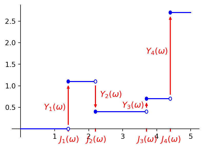
In addition to Brownian motion and Poisson processes, there is another fundamental family of processes that are also Lévy processes: a cousin of the, let’s admit it, somewhat plain and boring Poisson process namely compound Poisson processes. We create it by spicing up the Poisson process in one particular way. Recall (from Section 8.4) that a Poisson process with intensity \(\lambda>0\) has the following structure: at the (random) arrival times \(0<J_1<J_2< \ldots\), which are spaced apart by the i.i.d., \(\text{Exp}(\lambda)\) distributed interarrival times, a jump upwards of size \(1\) happens. If you don’t remember the details exactly, first quickly review Section 8.4 to have them sharp before reading the below.

Let’s just keep these arrival times as they are, but let’s make the jump sizes a bit more adventurous by allowing for them to be random. More precisely, on a probability space \((\Omega,\mathcal{F},\P)\) where a Poisson process \((N_t)_{t \geq 0}\) with intensity \(\lambda>0\) (and arrival times \(J_1, J_2, \ldots\)) lives, let \(Y_1, Y_2, \ldots\) be an i.i.d. (independent and identically distributed) sequence of random variables, also independent of \((N_t)_{t \geq 0}\). Create a new process \((X_t)_{t \geq 0}\) that is piecewise constant like \((N_t)_{t \geq 0}\), with \(X_0=0\), and which at time \(J_1\) has a jump of size \(Y_1\), at time \(J_2\) a jump of size \(Y_2\), etc. Note that, depending on the (common, because identically distributed) distribution that we give the jump sizes \(Y_1, Y_2, \ldots\), the jumps may well be negative/downwards as well as positive/upwards.

So if we look at this process from the path perspective, i.e. we fix an \(\omega \in \Omega\) — so that all the random variables that play a role take a value in \(\R\): the arrival times \(0<J_1(\omega)<J_2(\omega)<\ldots\) and jump sizes \(Y_1(\omega), Y_2(\omega), \ldots\) — and we consider the resulting path \(t \mapsto X_t(\omega)\), then we get to see something that looks like Figure 10.1.

Figure 10.1: In blue, a path \(t \mapsto X_t(\omega)\) of a compound Poisson process, with in red the random variables from which the path is constructed: the arrival/jump times \(0<J_1(\omega)<J_2(\omega)<J_3(\omega)<J_4(\omega)\) with jump sizes \(Y_1(\omega)=1.1\), \(Y_2(\omega)=-0.7\), \(Y_3(\omega)=0.3\) and \(Y_4(\omega)=2\). Compare and contrast this structure with that of a Poisson process, cf. Figure 8.2!

On the other hand (effectively equivalently of course), in order to write down an expression for the random variable \(X_t\) for any fixed time \(t>0\), observe that as the process only changes value/level when a jump happens and starts at value \(X_0=0\), the value/level at time \(t\) i.e. \(X_t\) is simply equal to the sum of all the jumps that happened up until (including) time \(t\). There are exactly \(N_t \in \{0,1,\ldots\}\) such jumps, of sizes \(Y_1, Y_2, \ldots, Y_{N_t}\), so that we can write \[X_t=Y_1+Y_2+\ldots+Y_{N_t}=\sum_{k=1}^{N_t} Y_k \quad \text{for all } t \geq 0, \tag{10.5}\] where we understand an “empty sum” i.e. \(\sum_{k=1}^{0}\) to equal \(0\).

If you are not entirely convinced yet that this is the right expression, then note that we can write Equation 10.5 out in the following way for any \(t>0\): \[X_t=\begin{cases} 0 & \text{if } N_t=0 \\ Y_1 & \text{if } N_t=1 \\ Y_1+Y_2 & \text{if } N_t=2 \\ \quad \vdots & \quad \vdots \end{cases} = \begin{cases} 0 & \text{if } t \in [0,J_1) \\ Y_1 & \text{if } t \in [J_1,J_2) \\ Y_1+Y_2 & \text{if } t \in [J_2,J_3) \\ \quad \vdots & \quad \vdots \end{cases} \tag{10.6}\] and now check for yourself that if you walk over the time axis in Figure 10.1, starting at time \(t=0\), then the value \(X_t\) has for any \(t \geq 0\) (well, at least until the end of the time axis in the visual) indeed coincides with the value that Equation 10.6 insists it should have.

It is worth noting that one valid choice for the jump sizes is to simply set them equal to \(1\) i.e. \(Y_1=Y_2=\ldots=1\). That particular choice puts us back to where we started from: the original Poisson process, because that one had jumps of size \(1\) to begin with. Indeed we can verify that from Equation 10.5 as well: \[X_t = \sum_{k=1}^{N_t} 1 = N_t \quad \text{for all } t \geq 0 \tag{10.7}\] i.e. our new process \((X_t)_{t \geq 0}\) simplifies to just \((N_t)_{t \geq 0}\). So Poisson processes belong to the family of compound Poisson processes as well.

Definition 10.3 On some probability space \((\Omega,\mathcal{F},\P)\), let \((N_t)_{t \geq 0}\) be a Poisson process with intensity \(\lambda>0\) and \(Y_1, Y_2, \ldots\) be a sequence of i.i.d. (independent and identically distributed) random variables, independent of \((N_t)_{t \geq 0}\).

Then the process \((X_t)_{t \geq 0}\) given by \[X_t=\sum_{k=1}^{N_t} Y_k \quad \text{for all } t \geq 0,\] where we understand an “empty sum” i.e. \(\sum_{k=1}^{0}\) to equal \(0\), is called a compound Poisson process.

Note that this process depends on two parameters/inputs: the intensity \(\lambda>0\), which governs the rate at which jumps arrive (recall from Section 8.4 that the expected waiting time between two arrivals is \(1/\lambda\)), and a distribution for the jump sizes \(Y_1, Y_2, \ldots\) which we could for instance represent by their common cdf (cf. Definition 2.6), say \(F_Y\).

We claimed at the start of this section that a compound Poisson process \((X_t)_{t \geq 0}\) is also a Lévy process — let’s check this via Definition 10.2. It’s clear that \(X_0=0\) a.s. — because in Equation 10.5 we have \(N_0=0\) a.s. (recall from Definition 8.4) so that we have a.s. an “empty sum” which we said we understand as having value \(0\) — and that it has cadlag paths (you see it in REF, and if you’d like a more precise argument reuse the one we also used in Section 8.4.1 for the cadlag property of our construction of a Poisson process). So it remains to check properties iii and iv from Definition 10.2.

For property iii, just observe that for any \(0 \leq t_1<t_2\), \[X_{t_2}-X_{t_1}=\sum_{k=1}^{N_{t_2}} Y_k - \sum_{k=1}^{N_{t_1}} Y_k=\sum_{k=N_{t_1}+1}^{N_{t_2}} Y_k\] and note that the number of terms in this sum is \(N_{t_2}-N_{t_1}\) which is independent of \(\{ N_s \, | \, s \in [0,t_1]\}\) (as first seen in Definition 8.4) and the jump sizes are all independent of each other. Further, since the jump sizes are i.i.d., this expression also shows that \(X_{t_2}-X_{t_1}\) has the same distribution as \[\sum_{k=1}^{N_{t_2}-N_{t_1}} Y_k\] (as both expressions sum the same number of jumps, the fact that the jump sizes are different elements from the sequence \(Y_1, Y_2, \ldots\) does not matter for the distribution as these are i.i.d.) which in turn has the same distribution as \[\sum_{k=1}^{N_{t_2-t_1}} Y_k=X_{t_2-t_1},\] since \(N_{t_2}-N_{t_1}\) has the same distribution as \(N_{t_2-t_1}\) (either explicitly find their distributions from Definition 8.4 and check that they are equal, or otherwise use that in Section 10.3 we have already seen that \((N_t)_{t \geq 0}\) is a Lévy process and hence it satisfies property iv of Definition 10.2). This confirms that property iv of Definition 10.2 also holds for \((X_t)_{t \geq 0}\).

Recall that in Proposition 10.2 we saw that every Lévy process has a characteristic exponent. Let’s find out what that guy looks like for a compound Poisson process \((X_t)_{t \geq 0}\), by working out the cf of \(X_1\): \[\varphi_{X_1}(z)=\E[e^{\mathrm{i}zX_1}].\] For this we need to work with \[X_1=\sum_{k=1}^{N_1} Y_k, \tag{10.8}\] which is a bit of head scratcher — a sum of a fixed number of i.i.d. random variables works very nicely with cf’s (recall Definition 10.1 iv) but a sum like the above one, with a random number of elements, is a different story!

However there is a nice and elegant way to deal with this issue, reaching back to our old friend the law of total expectation (if needs be, recall that we had him say hello in Exercise 4.4). For this, recall that \(N_1\) has range \(\{0,1,\ldots\}\) (cf. Definition 8.4) and hence the collection of events \(\{N_1=0\}\), \(\{N_1=1\}\), \(\ldots\) forms a partition of \(\Omega\). Plugging this into the law of total expectation, we can write \[\varphi_{X_1}(z)=\E[e^{\mathrm{i}zX_1}]=\sum_{n=0}^\infty \E[e^{\mathrm{i}zX_1} \, | \, N_1=n] \P(N_1=n). \tag{10.9}\] For any \(n=1,2,\ldots\) we can work out \[\begin{align*} \E [ e^{\mathrm{i}zX_1} \, | \, N_1=n] &= \E \left[ \exp \left( \mathrm{i}z \sum_{k=1}^n Y_k \right) \right] \\ &= \varphi_{Y_1+\ldots+Y_n}(z) \\ &= \varphi_{Y_1}(z) \varphi_{Y_2}(z) \cdots \varphi_{Y_n}(z) \\ &= \big( \varphi_{Y_1}(z) \big)^n, \end{align*} \tag{10.10}\] where the first equation uses that conditional on \(\{N_1=n\}\), \(X_1\) can be replaced by \(\sum_{k=1}^n Y_k\) (cf. Equation 10.8), the second is just by def, the third uses that \(Y_1, \ldots, Y_n\) are independent (cf. Definition 10.3) so that we can apply Definition 10.1 iv, and the final one that \(Y_1, \ldots, Y_n\) all have the same distribution (cf. Definition 10.3) and hence the same cf. Observe that Equation 10.10 is also true for \(n=0\), as in that case both sides equal \(1\).

Plugging Equation 10.10 into Equation 10.9, we can work out, along the same lines as in Exercise 10.2 (i.e. using the pmf of \(N_1 \sim \text{Poisson}(\lambda)\) as well as the power series of the exponential) \[\begin{align*} \varphi_{X_1}(z) &= \sum_{n=0}^\infty \big( \varphi_{Y_1}(z) \big)^n \P(N_1=n) \\ &= \sum_{n=0}^\infty \big( \varphi_{Y_1}(z) \big)^n \frac{\lambda^n}{n!} e^{-\lambda} \\ &= e^{-\lambda} \sum_{n=0}^\infty \frac{\big( \varphi_{Y_1}(z) \big)^n}{n!} \\ &= e^{-\lambda} \exp \left( \lambda \varphi_{Y_1}(z) \right) \\ &= \exp \left( \lambda \left( \varphi_{Y_1}(z)-1 \right) \right). \end{align*} \] Finally, we have now done the hard work needed to derive the characteristic exponent of \((X_t)_{t \geq 0}\), cf. Proposition 10.2: \[\Psi(z)=-\log \left( \varphi_{X_1}(z) \right)=\lambda \left( 1-\varphi_{Y_1}(z) \right).\]

Let’s put the conclusions of all of this together:

Proposition 10.4 A compound Poisson process \((X_t)_{t \geq 0}\) as defined in Definition 10.3 is a Lévy process with characteristic exponent \[\Psi(z)=\lambda \left( 1-\varphi_{Y_1}(z) \right) \quad \text{for all } z \in \R.\] Note that both parameters of the process, the intensity \(\lambda\) and the distribution of the jump sizes (via the cf of \(Y_1\)) appear in this expression, as you would expect of course.

Remark 10.3. If you find the argument we used to justify the first line in Equation 10.10 a bit too wishy-washy, here is a more detailed one! Recall from the def of conditioning on an event (cf. Definition 4.1) that \[\E [ e^{\mathrm{i}zX_1} \, | \, N_1=n]=\frac{1}{\P(N_1=n)} \E \left[ \mathbf{1}_{\{N_1=n\}} e^{\mathrm{i}zX_1} \right]. \tag{10.11}\] Now observe that for any \(\omega \in \Omega\), using that \[\mathbf{1}_{\{N_1=n\}}(\omega)=1 \iff N_1(\omega)=n,\] we have from Equation 10.8 \[\mathbf{1}_{\{N_1=n\}}(\omega) e^{\mathrm{i}zX_1(\omega)} = \mathbf{1}_{\{N_1=n\}}(\omega) e^{\mathrm{i}z (Y_1(\omega)+\ldots+Y_n(\omega))}.\] So the random variables on both sides in particular also have the same expectation, and since \(N_1\) is independent of \(Y_1, \ldots, Y_n\) we can also use Proposition 3.6 viii to get \[\begin{align*} \E \left[ \mathbf{1}_{\{N_1=n\}} e^{\mathrm{i}zX_1} \right] &= \E \left[ \mathbf{1}_{\{N_1=n\}} e^{\mathrm{i}z(Y_1+\ldots+Y_n)} \right] \\ &= \E \left[ \mathbf{1}_{\{N_1=n\}} \right] \E \left[ e^{\mathrm{i}z(Y_1+\ldots+Y_n)} \right] \\ &= \P(N_1=n) \E \left[ e^{\mathrm{i}z(Y_1+\ldots+Y_n)} \right], \end{align*} \] and now just plug this back into Equation 10.11.

Finally in this section, we have previously seen that if we take a linear combination of two independent Lévy processes that we get another Lévy process (cf. Proposition 10.1) — it’s a nice and easy way of creating new Lévy processes from existing ones. So if we take a linear combination of two independent compound Poisson processes, we will get a Lévy process. But what kind exactly? Well, as it turns out, another compound Poisson process! Note, just for interest, that this is a generalisation of Exercise 8.9.

Proposition 10.5 On some probability space, let \((X^{(1)}_t)_{t \geq 0}\) and \((X^{(2)}_t)_{t \geq 0}\) be two independent compound Poisson processes, with intensities \(\lambda^{(1)}>0\) and \(\lambda^{(2)}>0\) and jump size distributions represented by the cdf’s \(F^{(1)}\) and \(F^{(2)}\) resp. For constants \(a,b >0\), define the process \((X^{(3)}_t)_{t \geq 0}\) as \[X^{(3)}_t=a X^{(1)}_t+b X^{(2)}_t \quad \text{for all } t \geq 0.\] Then \((X^{(3)}_t)_{t \geq 0}\) is (has the same law as) a compound Poisson process with intensity \(\lambda^{(1)}+\lambda^{(2)}\) and jump size distribution represented by the cdf \(F\) given by \[F(x)=\frac{\lambda^{(1)} F^{(1)}(x/a)+\lambda^{(2)} F^{(2)}(x/b)}{\lambda^{(1)}+\lambda^{(2)}} \quad \text{for all } x \in \R. \tag{10.12}\]

Note: this result remains true for any \(a,b \in \R\) as long as at least one of them is not \(0\):

• if \(b=0\) then \((X^{(3)}_t)_{t \geq 0}\) is just \((X^{(1)}_t)_{t \geq 0}\) with its jump sizes mutiplied by a factor \(a\),
• if one or both of \(a,b\) is strictly negative, then the result remains the same except for Equation 10.12, now the distribution of the jump sizes of \((X^{(3)}_t)_{t \geq 0}\) is best described by their common cf: \[\varphi(z)=\lambda^{(1)} \left( 1- \varphi^{(1)}(az) \right) + \lambda^{(2)} \left( 1- \varphi^{(2)}(bz) \right) \quad \text{for all } z \in \R,\] where \(\varphi^{(1)}\) and \(\varphi^{(2)}\) are the cf’s of the jump size distributions of \((X^{(1)}_t)_{t \geq 0}\) and \((X^{(2)}_t)_{t \geq 0}\) resp.

Proof. We know from Proposition 10.1 that \((X^{(3)}_t)_{t \geq 0}\) is a Lévy process, so its law is fully determined by its characteristic exponent (cf. Remark 10.2). We break the proof up in two steps: first we find the characteristic exponent of \((X^{(3)}_t)_{t \geq 0}\) from its definition, and then we find the characteristic exponent of the compound Poisson process introduced in the statement and conclude that they are equal, so that the claim follows (also recall Remark 10.2).

Denote the jump sizes of \((X^{(1)}_t)_{t \geq 0}\) by \(Y^{(1)}_1, Y^{(1)}_2, \ldots\) (with common cdf \(F^{(1)}\)) and those of \((X^{(2)}_t)_{t \geq 0}\) by \(Y^{(2)}_1, Y^{(2)}_2, \ldots\) (with common cdf \(F^{(2)}\)).

Step 1. In order to find an expression for the characteristic exponent of \((X^{(3)}_t)_{t \geq 0}\), let’s work out the cf of the random variable \(X^{(3)}_1\) first: observe that for any \(z \in \R\) \[\begin{align*} \E \left[ \exp \left( \mathrm{i}z X^{(3)}_1 \right) \right] &= \E \left[ \exp \left( \mathrm{i}z (a X^{(1)}_1+b X^{(2)}_1) \right) \right] \\ &= \E \left[ \exp \left( \mathrm{i}z a X^{(1)}_1 \right) \exp \left( \mathrm{i}z b X^{(2)}_1 \right) \right] \\ &= \E \left[ \exp \left( \mathrm{i}z a X^{(1)}_1 \right) \right] \E \left[ \exp \left( \mathrm{i}z b X^{(2)}_1 \right) \right], \end{align*} \] where the final equality uses the independence of \(a X^{(1)}_1\) and \(b X^{(2)}_1\) (cf. Definition 10.1 iv). So, denoting by \(\varphi^{(k)}\) the cf of \(X^{(k)}_1\) for \(k=1,2,3\), this shows that we have \[\varphi^{(3)}(z)=\varphi^{(1)}(az) \varphi^{(2)}(bz) \quad \text{for all } z \in \R.\] Denoting by \(\Psi^{(k)}\) the characteristic exponent of the three processes (cf. Proposition 10.2) for \(k=1,2,3\), by taking \(-\log()\) of both sides of the above equation we readily get the following relationship: \[\Psi^{(3)}(z)=\Psi^{(1)}(az)+\Psi^{(2)}(bz) \quad \text{for all } z \in \R.\] Plugging in the result from Proposition 10.4, we wrap this first step up with \[\Psi^{(3)}(z)=\lambda^{(1)} \left( 1-\varphi_{Y^{(1)}_1}(az) \right)+\lambda^{(2)} \left( 1-\varphi_{Y^{(2)}_1}(bz) \right) \quad \text{for all } z \in \R. \tag{10.13}\]

Step 2. Now let \((Z_t)_{t \geq 0}\) be a compound Poisson process with intensity \(\lambda^{(1)}+\lambda^{(2)}\) and jump sizes \(\xi_1, \xi_2, \ldots\) given by \[\xi_k=a (1-U_k) Y^{(1)}_k + b U_k Y^{(2)}_k \quad \text{for all } k=1,2,\ldots, \tag{10.14}\] where \(U_1, U_2, \ldots\) are i.i.d. random variables (also independent of all else) with the following common distribution: \[\P(U_k=0)=\frac{\lambda^{(1)}}{\lambda^{(1)}+\lambda^{(2)}} \quad \text{and} \quad \P(U_k=1)=\frac{\lambda^{(2)}}{\lambda^{(1)}+\lambda^{(2)}}. \tag{10.15}\] We will see in Exercise 10.6 that the common cdf of the \(\xi_k\)’s is Equation 10.12, and that the Laplace exponent of this process equals Equation 10.13. This wraps up the proof.

Remark 10.4. The above proof also reveals a quite nice interpretation of the sum process \((X^{(3)}_t)_{t \geq 0}\)! Taking \(a=b=1\):

• It has intensity \(\lambda^{(1)}+\lambda^{(2)}\) i.e. in a time interval \([0,t]\) the number of jumps is \(\text{Poisson}((\lambda^{(1)}+\lambda^{(2)})t)\) distributed, so (in distribution) \((X^{(3)}_t)_{t \geq 0}\) has as many jumps in the time interval \([0,t]\) as \((X^{(1)}_t)_{t \geq 0}\) and \((X^{(2)}_t)_{t \geq 0}\) have jointly.
• Each time \((X^{(3)}_t)_{t \geq 0}\) has a jump, Equation 10.14 shows that we can imagine the jump size to be determined as follows: consider a coin that yields Heads with prob \(\lambda^{(1)}/(\lambda^{(1)}+\lambda^{(2)})\) and Tails with prob \(\lambda^{(2)}/(\lambda^{(1)}+\lambda^{(2)})\), toss it and take a jump size from \((X^{(1)}_t)_{t \geq 0}\) resp. \((X^{(2)}_t)_{t \geq 0}\) if Heads resp. Tails.

So, roughly speaking: the first bullet point illustrates that \((X^{(3)}_t)_{t \geq 0}\) has enough jumps to cover all the jumps of both \((X^{(1)}_t)_{t \geq 0}\) and \((X^{(2)}_t)_{t \geq 0}\), and the second bullet point shows that the sizes of these jumps are a mix: sometimes from \((X^{(1)}_t)_{t \geq 0}\) and sometimes from \((X^{(2)}_t)_{t \geq 0}\), in exactly the right ratio to reflect how many jumps \((X^{(1)}_t)_{t \geq 0}\) has vs \((X^{(2)}_t)_{t \geq 0}\)!

For other choices of \(a,b\) this interpretation stays the same, it’s just that then in the second bullet point above, a jump size is also scaled by a factor \(a\) resp. \(b\) if it comes from \((X^{(1)}_t)_{t \geq 0}\) resp. \((X^{(2)}_t)_{t \geq 0}\).

Exercises

You can now do Exercise 10.4–Exercise 10.6.

10.6 Jump diffusions

In Section 10.3 we saw that a Brownian motion is a Lévy process, as is the trivial deterministic process that increases linearly. Further we have discussed the family of compound Poisson processes, generalising Poisson processes, in the above Section 10.5 as further examples of Lévy processes. Taking a linear combination of such guys we again get a Lévy process (cf. Proposition 10.1), and this brings us to the class of jump diffusions.

Definition 10.4 On a probability space, let \((B_t)_{t \geq 0}\) be a Brownian motion and \((Z_t)_{t \geq 0}\) a compound Poisson process independent of \((B_t)_{t \geq 0}\), with intensity \(\lambda>0\) and jump size distribution represented by a cdf \(F\). Further let \(\sigma>0\) and \(a \in \R\) be constants.

Then the Lévy process \((X_t)_{t \geq 0}\) given by \[X_t = \sigma B_t + a t + Z_t \quad \text{for all } t \geq 0 \tag{10.16}\] is called a jump diffusion, with parameters \(\sigma>0\), \(a \in \R\), \(\lambda>0\) and \(F\). Its characteristic exponent is given by \[\Psi(z)=\frac{\sigma^2}{2}z^2-\mathrm{i}az + \lambda \left( 1-\varphi(z) \right) \quad \text{for all } z \in \R,\] where \(\varphi\) is the cf of the jump sizes of \((Z_t)_{t \geq 0}\).

Note that the expression for the characteristic exponent immediately follows from the independence of the three components and Example 10.3 & Proposition 10.4.

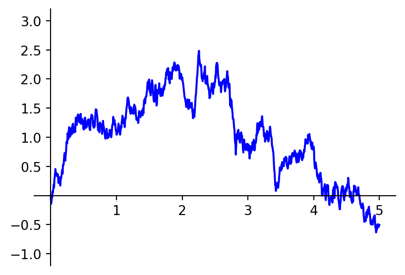
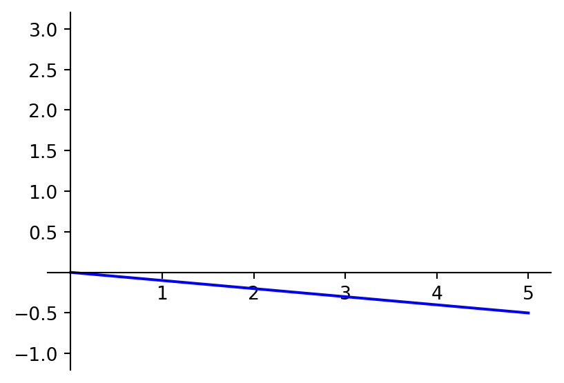
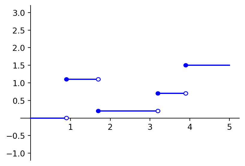
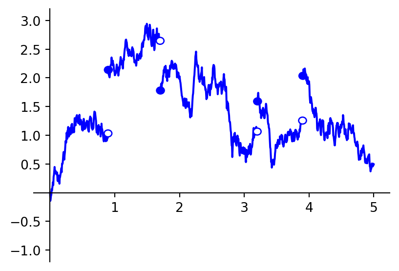
As Equation 10.16 shows, for some \(\omega \in \Omega\) a path \(t \mapsto X_t(\omega)\) of a jump diffusion consists of the sum of three paths(/functions): the characteristically spiky path \(t \mapsto \sigma B_t(\omega)\) (typically called the Brownian part), where the parameter \(\sigma\) allows for some scaling of the Brownian path; plus a linear trend \(t \mapsto a t\) (often called the drift); plus the path of a compound Poisson process \(t \mapsto Z_t(\omega)\) which introduces jumps into the resulting sum path (hence the jump part), the intensity of which can be controlled by \(\lambda>0\) and the jump sizes by \(F\). See also Figure 10.2.

(a) A path of a scaled Brownian motion \(t \mapsto \sigma B_t(\omega)\) (in this case \(\sigma=1\))

(b) A path of the drift \(t \mapsto at\) (in this case \(a=-0.5\))

(c) A path of a compound Poisson process \(t \mapsto Z_t(\omega)\) (in this case with Normally distributed jumps, so both positive and negative jumps are possible)

(d) The resulting path of the jump diffusion \((X_t)_{t \geq 0}\): \(t \mapsto X_t(\omega)=\sigma B_t(\omega)+at+Z_t(\omega)\)

Figure 10.2: A path of a jump diffusion \((X_t)_{t \geq 0}\) as put together from its three components

Altogether this makes jump diffusions a popular subclass of Lévy processes: they are quite tractable while also being very flexible in the sense that they can show a range of different behaviours (and hence model a large variety of phenomena).

For example in financial maths, the seminal Black&Scholes model uses a geometric Brownian motion to model the evolution of the price of an asset (e.g. a stock) over time i.e. a process \((S_t)_{t \geq 0}\) of the form \[S_t=S_0 e^{\sigma B_t + a t} \quad \text{for all } t \geq 0, \tag{10.17}\] where \(S_0>0\) (the observed price at time \(0\)), \(\sigma>0\) and \(a \in \R\) are parameters. This model (and in particular the theory around it, allowing to assess and protect against the risk involved with trading in financial instruments such as options) was the bedrock of modern financial maths some 40 years ago. Nevertheless it has some limitations. Notably, if you apply some statistical analysis then it turns out that observed historical stock price movements do not fit Equation 10.17 as well as you would ideally like.

Hence a lot of research has gone into finding alternative models that do not suffer from that problem, but on the other hand keep the beautiful option pricing theory included with the Black&Scholes model as much as possible in tact. A natural direction to look into is a model of the form \[S_t=S_0 e^{X_t} \quad \text{for all } t \geq 0\] for some different Lévy process \((X_t)_{t \geq 0}\) than the Brownian motion with drift used in Equation 10.17. And within such models, a natural first step is to look at using a jump diffusion for \((X_t)_{t \geq 0}\). Some prominent examples are jump diffusions with Normally distributed jumps (the Merton model) and with two-sided Exponentially distributed jumps (the Kou model), see e.g. Section 4.3 in Tankov (2003) if you’d like to read a bit more about these models. More of this in the next semester course Stochastic Modelling in Finance!

Exercises

You can now do Exercise 10.7.

10.7 General Lévy processes (non-examinable)

Finally in this chapter, a quick look at what a Lévy process looks like in general — though the jump diffusions from the above Section 10.6 form a very useful subclass, far from every possible Lévy process is of this form!

As a first step, let’s think about what form the characteristic exponent of Lévy processes can have. For this, observe that for a Lévy process \((X_t)_{t \geq 0}\) on some probability space \((\Omega,\mathcal{F},\P)\) we can trivially write for any integer \(n=2,3,\ldots\) \[X_1-X_0=\sum_{k=1}^n \left( X_{k/n}-X_{(k-1)/n} \right) \tag{10.18}\] (pointwise). Note that in the right hand side of this equation we have a sum of increments which are independent (cf. Definition 10.2 iii) and all have the same distribution as \(X_{1/n}\) (cf. Definition 10.2 iv) so in particular also as each other. Note that on the left hand side, \(X_1-X_0\) has the same distribution as \(X_1\) (by Definition 10.2 i & Exercise 2.9).

So what Equation 10.18 is telling us is the following: \(X_1\) is equal in distribution to a sum of \(n\) i.i.d.¹ random variables (we know from the above that we can take these random variables to be \(n\) independent copies of \(X_{1/n}\) but that is irrelevant here) — and this is not just true for some \(n=2,3,\ldots\), this is true for all \(n=2,3,\ldots\)! This is quite special! We call such distributions infinitely divisible.

¹ Recall: independent and identically distributed

² If you think about it, Normal and Poisson are immediately clear since we already know that Brownian motion and Poisson processes are Lévy processes!

³ Note that the integral here is “just” a Lebesgue integral as discussed in Chapter 3!

Some well known examples of infinitely divisible distributions are Normal, Poisson, stable, inverse Gaussian and Cauchy distributions². But of course there are also many infinitely divisible distributions that are not known by a flashy name. The impressive Lévy-Khintchine formula (see e.g. Theorem 1.3 in Kyprianou (2014)) gives us a full characterisation: a distribution is infinitely divisible if and only if its cf \(\varphi\) can be expressed as \[\varphi(z)=e^{-\Psi(z)} \quad \text{for all } z \in \R,\] where \(\Psi\) is of the following form³: \[\Psi(z)=\frac{\sigma^2}{2}z^2 + \mathrm{i}az + \int_{(-\infty,\infty)} \left( 1-e^{\mathrm{i}zx}+\mathbf{1}_{\{ \lvert x \rvert <1\}} \mathrm{i}zx \right) \, \Pi(dx). \tag{10.19}\] This expression contains the following parameters: \(\sigma \geq 0\), \(a \in \R\), and \(\Pi\) is a measure on \(\R\) with \(\Pi(\{0\})=0\) satisfying \[\int_{(-\infty,\infty)} \min\{1,x^2\} \, \Pi(dx)<\infty \tag{10.20}\] called the Lévy measure of this distribution. These three parameters put together, i.e. \((\sigma,a,\Pi)\) is called a Lévy triplet.

Comparing this with our definition of the characteristic exponent of a Lévy process (cf. Proposition 10.2), we arrive at the following conclusion: if \((X_t)_{t \geq 0}\) is a Lévy process, then its characteristic exponent \(\Psi\) must be of the form Equation 10.19. Indeed all specific examples of characteristic exponents we have encountered so far in this chapter fit this form!

The reverse implication is also true, this is the at least equally impressive Lévy-Itô decomposition (see e.g. Theorem 2.1 in Kyprianou (2014)): for any choice of parameters \((\sigma,a,\Pi)\) (satisfying the above assumptions) there exists a probability space \((\Omega,\mathcal{F},\P)\) and a process \((X_t)_{t \geq 0}\) which is a Lévy process with characteristic exponent given by Equation 10.19. In fact the Lévy-Itô decomposition tells us a little bit more, namely how to construct \((\Omega,\mathcal{F},\P)\) and \((X_t)_{t \geq 0}\).

To illustrate this construction briefly, define \(C=(-\infty,-1) \cup (1,\infty)\) and observe that it follows from Equation 10.20 that \[\Pi(C)=\int_C 1 \, \Pi(dx) \leq \int_{(-\infty,\infty)} \min\{1,x^2\} \, \Pi(dx)<\infty. \tag{10.21}\] Assuming that \(\Pi(C)>0\), consider the scaled measure \(\mu(B):=\Pi(B \cap C)/\Pi(C)\) for all Borel sets \(B \subseteq \R\). Note that \(\mu(\R)=\Pi(\R \cap C)/\Pi(C)=1\) i.e. \(\mu\) is actually a probability measure on \(\R\) (recall from Definition 2.5) and hence a random variable, say \(\xi\), exists with this \(\mu\) as its distribution (cf. e.g. Exercise 2.7). Let \((Z_t)_{t \geq 0}\) be a compound Poisson process with intensity \(\Pi(C)\) and jump size distribution \(\mu\) i.e. as jumps sizes independent copies of \(\xi\). (If \(\Pi(C)=0\), then let \((Z_t)_{t \geq 0}\) simply be the trivial process identically equal to \(0\).)

The construction in the Lévy-Itô decomposition tells us that if we take a Brownian motion \((B_t)_{t \geq 0}\) independent of \((Z_t)_{t \geq 0}\) as well as a third independent process \((M_t)_{t \geq 0}\) so that the sum process \((X_t)_{t \geq 0}\) given by \[X_t = \sigma B_t - at + Z_t + M_t \quad \text{for all } t \geq 0 \tag{10.22}\] is indeed a Lévy process corresponding to the given triplet \((\sigma,a,\Pi)\)! If we put our finger on that \((M_t)_{t \geq 0}\) for a moment, then we see here nothing but a jump diffusion as discussed in Section 10.6 (unless \(\Pi(C)=0\), then it is just a Brownian motion with drift).

So what is exactly that final ingredient, that process \((M_t)_{t \geq 0}\)?? To partly answer this, first note that the above construction of \((Z_t)_{t \geq 0}\) would not necessarily have worked if we had tried it with \(C=\R\): it is quite well possible that \(\Pi(\R)=\infty\) and so the scaling argument wouldn’t have worked. What this reflects is the following. The Lévy measure \(\Pi\) describes the “jump structure” of the corresponding Lévy process: for any Borel set \(B \subseteq \R \setminus \{0\}\), \(\Pi(B)\) is the expected number of jumps of size in \(B\) the process experiences in a unit time interval i.e. \[\Pi(B)=\E \left[ \# \{ t \in [0,1] \, | \, X_t-X_{t-} \in B \} \right],\] where \(X_{t-}\) denotes the left hand limit in time \(t\) i.e. \[X_{t-} := \lim_{s \uparrow t} X_s\] and \(\# A\) denotes the number of elements in a set \(A\).

So Equation 10.21 tells us that the expected number of jumps of absolute value larger than \(1\) in a unit time interval is finite, and hence in particular this number of jumps is finite a.s.⁴ This allows us to represent these jumps in the form of the compound Poisson process \((Z_t)_{t \geq 0}\)⁵. But it may well be true that \(\Pi([-1,1])=\infty\) i.e. a Lévy process can have an infinite number of “small” jumps i.e. of absolute size at most \(1\) in a unit time interval! This is fundamentally incompatible with the structure that a compound Poisson process (and a jump diffusion) has. Lévy processes with this feature are said to be of infinite activity and to represent such behaviour in our decomposition Equation 10.22 we need that somewhat secretive extra ingredient \((M_t)_{t \geq 0}\). The construction of this process (from a given \(\Pi\)) is not very straightforward and it can generally only be characterised as a limit within the space of square integrable cadlag martingales starting from \(0\) (and has itself these properties). See e.g. Chapter 2 in Kyprianou (2014).

⁴ If you think about it, this property also follows from the cadlag property of the paths

⁵ The number of jumps that a compound Poisson process with intensity \(\lambda>0\) has in a unit time interval is (of course!) given by a \(\text{Poisson}(\lambda)\) distribution which is necessarily finite

This feature also illustrates that the class of Lévy processes is quite a bit richer than “just” the class of jump diffusions, and in particular it makes for some rather surprising and fascinating behaviour!

Besides the characterisation of the characteristic exponent of a Lévy process and the resulting understanding of what its building blocks are (as outlined in Equation 10.22), another property that all Lévy processes have and is crucial in their study is the strong Markov property. This is, loosely speaking, the stationary independent increment property on steroids. Fixing any time point \(s \geq 0\), we know that for any \(t \geq 0\) the increment \(X_{t+s}-X_s\) is independent of anything that happened up until time \(s\) and has the same distribution as \(X_{t-s}\). Indeed in fact, standing at time \(s\), considering how the process will evolve from that time onwards i.e. \((X_{t+s}-X_s)_{t \geq 0}\) is independent of what has happened so far and has the same law as \((X_t)_{t \geq 0}\) itself. The strong Markov property entails that this is even true if we replace \(s\) by a stopping time (provided we’re working with a suitable filtration etc.). For instance, we could take the first time that our process enters a set \([a,\infty)\) — if we consider the evolution of the process from that time onwards then this behaves just like a new, independent copy of our process! See e.g. Theorem 3.1 in Kyprianou (2014).

I really have to stop typing at some point though (unfortunately that’s always when there’s more beautiful stuff just around the corner of course…) — if you’re interested in more Lévy processes, then have a look at any of the books mentioned in Section 10.1!

10.8 Some exercises

About the exercises

Each exercise has a (rough) indication of its difficulty, as follows:

*	easier: can be solved by (almost) only using relevant definitions/results,
**	medium: in addition to relevant definitions/results, needs a limited amount of work/creativity,
***	harder: in addition to relevant definitions/results, needs a larger amount of work/serious creativity,
💀	warning: might make your brain hurt! These are mainly intended to provide some extra challenge for those of you keen on that and are generally quite hard. You don't need to worry about these too much for exam purposes.

The exam consists of mostly ** and *** level questions, some *, and possibly at most a few marks worth of 💀.

A bit of preaching: it is an incredibly important part of the study process to try and work on the exercises as much as possible. To become a better mathematician/learn new maths (and also to get a good exam mark ;)), above all you need to do it. And yes, of course that includes falling over things, and making mistakes, and getting stuck, and getting frustrated — all part of the game and what you’re supposed to be doing! Your lecturers have done that as well and still do it. What matters is that you don’t let that discourage you and that you make good use of the help and resources available to help you develop your skills. As part of that, many exercises have a hint in a block like this:

Hint (click to view)

Hint!

These are trying to help you on your way if you don’t know where to start or to provide some ideas if you get stuck. In spirit of the above, always have a look at these first and try again before you look at the full solution. (These hints are an extra service that won’t be available in the exam I’m afraid ;).)

Of course, we have our classes and there’s office hours, email etc. as well — I’m at any time very happy to help you with any questions you may have, and you should please never feel that any question is “too dumb” to ask!

Full/detailed solutions for the exercises will become available, just immediately below the exercises, after our Friday tutorial.

Exercise 10.1 [*/**] On some probability space \((\Omega,\mathcal{F},\P)\), let \(X\) be a constant random variable and \(Y\) any other random variable. Show that \(X\) and \(Y\) are independent (if needs be, recall Section 2.6.1).

Hint (click to view)

Recall from Section 2.6.1 that we need to show that for any Borel sets \(B_1, B_2 \in \mathcal{B}(\R)\) it holds that \[\P(X \in B_1 \ \& \ Y \in B_2)=\P(X \in B_1) \P(Y \in B_2).\] Now, if \(X\) is constant i.e. for some \(c \in \R\), \(X(\omega)=c\) for all \(\omega \in \Omega\), then it is not very hard to simplify both sides of the above equation and check they are indeed equal. For this, you may want to consider the cases \(c \in B_1\) and \(c \not\in B_1\) separately — in the former you should find that both sides equal \(\P(Y \in B_2)\) while in the latter case you should find that both sides equal \(0\).

Full solution (click to view)

Let \(c \in \R\) be the constant value that \(X\) takes i.e. \(X(\omega)=c\) for all \(\omega \in \Omega\). Recall from Section 2.6.1 that \(X\) and \(Y\) are independent if and only if for any Borel sets \(B_1, B_2\) we have that \[\P(X \in B_1 \ \& \ Y \in B_2)=\P(X \in B_1) \P(Y \in B_2). \tag{10.23}\] In order to show this, take any Borel sets \(B_1, B_2\) and let’s simply work out both sides of the above equation. Key is to realise(/recall from Section 2.3) that the event/inverse image \(\{X \in B_1\}=X^{-1}(B_1)\), in “full” notation \[\{ \omega \in \Omega \, | \, X(\omega) \in B_1 \}\] can be easily simplified: if \(c \in B_1\) then \(\{X \in B_1\}=\Omega\) while if \(c \not\in B_1\) then \(\{X \in B_1\}=\emptyset\).

Now, if \(B_1\) is such that \(c \in B_1\) then \[\{X \in B_1\} \cap \{Y \in B_2\}=\Omega \cap \{Y \in B_2\}=\{Y \in B_2\}\] i.e. \(\P(X \in B_1 \ \& \ Y \in B_2)=\P(Y \in B_2)\) and also \[\P(X \in B_1) \P(Y \in B_2)=\P(\Omega) \P(Y \in B_2)= 1 \cdot \P(Y \in B_2)=\P(Y \in B_2).\]

On the other hand, if \(B_1\) is such that \(c \not\in B_1\) then \[\{X \in B_1\} \cap \{Y \in B_2\}=\emptyset \cap \{Y \in B_2\}=\emptyset\] i.e. \(\P(X \in B_1 \ \& \ Y \in B_2)=\P(\emptyset)=0\) and also \[\P(X \in B_1) \P(Y \in B_2)=\P(\emptyset) \P(Y \in B_2)= 0 \cdot \P(Y \in B_2)=0.\]

So indeed Equation 10.23 holds in all cases!

Exercise 10.2 [**] On some probability space \((\Omega,\mathcal{F},\P)\), let \((B_t)_{t \geq 0}\) be a Brownian motion and \((N_t)_{t \geq 0}\) a Poisson process with intensity \(\lambda>0\). Recall from Example 10.1 that these are both Lévy processes.

1. Show that the characteristic exponent (cf. Proposition 10.2) of \((B_t)_{t \geq 0}\) is given by \[\Psi(z)=\frac{1}{2} z^2 \quad \text{for all } z \in \R.\]

   Hint: you may use that for any \(a \in \R\) it holds that \[\int_{-\infty}^\infty e^{-(x - \mathrm{i}a)^2/2} \d x=\sqrt{2\pi},\] consider finding a way to make use of this in your computation of the cf of \(B_1\)!

2. Next show that the characteristic exponent of \((N_t)_{t \geq 0}\) is given by \[\Psi(z)=\lambda (1-e^{\mathrm{i}z}) \quad \text{for all } z \in \R.\]

   Hint: recall that the power series of the exponential remains valid(/is typically used as definition) for complex numbers: \[e^x=\sum_{k=0}^\infty \frac{x^k}{k!} \quad \text{for all } x \in \C.\]

3. Finally, show that the characteristic exponent of the Lévy process defined in Example 10.2 is given by \[\Psi(z)=\frac{a^2}{2}z^2-\mathrm{i}zc+\lambda (1-e^{\mathrm{i}zb}) \quad \text{for all } z \in \R.\]

Hint (click to view)

For part i, just work out the cf of \(B_1\) i.e. \(\E[e^{\mathrm{i}zB_1}]\) as an integral (cf. Equation 2.8) and use the good old “completing the square” for instance to get it into a form that allows you to use the hint.

For part ii, again just work out the cf of \(N_1\) i.e. \(\E[e^{\mathrm{i}zN_1}]\) but in this case it becomes a summation (cf. Equation 2.6). A little bit of algebra, noting that \(\exp(\mathrm{i}zk)=\exp(\mathrm{i}z)^k\) and usng the hint should get you there without too much sweat!

For part iii, all you really need to do is work out the cf of \(Z_1\) a bit and make use of the independence (recall Definition 10.1 iv). Note that if a rv \(X\) has cf \(\varphi\), then (trivially!) the rv \(aX\) for a constant \(a\) has cf \(z \mapsto \varphi(az)\)!

Full solution (click to view)

For part i, recall from Definition 8.2 that \(B_1 \sim \mathcal{N}(0,1)\). So using the standard formula for the expectation of a function of a continuous rv (cf. Equation 2.8 via Proposition 3.5) and recalling the pdf of a \(\mathcal{N}(0,1)\) distribution (or picking it up from Wikipedia or so if needs be), we can work out the cf of \(B_1\) as \[\begin{align*} \varphi(z) &= \E[e^{\mathrm{i}zB_1}] \\ &= \int_{-\infty}^\infty e^{\mathrm{i}zx} \frac{1}{\sqrt{2\pi}} e^{-x^2/2} \d x \\ &= \frac{1}{\sqrt{2\pi}} \int_{-\infty}^\infty e^{-x^2/2 + \mathrm{i}zx} \d x \\ &= e^{-z^2/2} \frac{1}{\sqrt{2\pi}} \int_{-\infty}^\infty e^{-(x - \mathrm{i}z)^2/2} \d x \\ &= e^{-z^2/2}, \end{align*} \] where the final equality uses the hint. So we indeed get from Proposition 10.2 that the characteristic exponent is \[\Psi(z)=-\log(\varphi(z))=z^2/2.\]

For part ii, recall from Definition 8.4 that \(N_1 \sim \text{Poisson}(\lambda)\). So using the standard formula for the expectation of a function of a discrete rv (cf. Equation 2.6 via Proposition 3.5) and recalling the pmf of a \(\text{Poisson}(\lambda)\) distribution (or picking it up from Wikipedia or so if needs be), we can work out the cf of \(N_1\) as \[\begin{align*} \varphi(z) &= \E[e^{\mathrm{i}zN_1}] \\ &= \sum_{k=0}^\infty e^{\mathrm{i}zk} \P(N_1=k) \\ &= \sum_{k=0}^\infty e^{\mathrm{i}zk} \frac{\lambda^k}{k!} e^{-\lambda} \\ &= e^{-\lambda} \sum_{k=0}^\infty \frac{\left( \lambda e^{\mathrm{i}z}\right)^k}{k!} \\ &= e^{-\lambda} e^{\lambda e^{\mathrm{i}z}} \\ &= e^{\lambda (e^{\mathrm{i}z}-1)}, \end{align*} \] where the fifth equality uses the hint. Now we can again find the required characteristic exponent using its def from Proposition 10.2: \[\Psi(z)=-\log(\varphi(z))=\lambda (1-e^{\mathrm{i}z}).\]

For part iii, first working out the cf of \(Z_1\): \[\begin{align*} \E[e^{\mathrm{i}zZ_1}] &= \E[e^{\mathrm{i}z(aB_1+bN_1+c)}] \\ &= \E[e^{\mathrm{i}zaB_1} e^{\mathrm{i}zbN_1}] e^{\mathrm{i}zc} \\ &= \E[e^{\mathrm{i}zaB_1}] \E[e^{\mathrm{i}zbN_1}] e^{\mathrm{i}zc} \\ &= e^{-a^2z^2/2} e^{\lambda (e^{\mathrm{i}zb}-1)} e^{\mathrm{i}zc} \\ &= e^{-a^2z^2/2+\lambda (e^{\mathrm{i}zb}-1)+\mathrm{i}zc}, \end{align*} \] where the third line uses the assumed independence of \(B_1\) and \(N_1\) (cf. Definition 10.1 iv) and the fourth line uses the results from parts i and ii (note that we plug \(az\) as argument into the cf from part i, and similarly \(bz\) in part ii). Finally again use the def from Proposition 10.2.

Exercise 10.3 [*/**] On some probability space \((\Omega,\mathcal{F},\P)\), let \((B_t)_{t \geq 0}\) be a Brownian motion and \((N_t)_{t \geq 0}\) a Poisson process with intensity \(\lambda>0\), independent of each other. Further consider the process \((X_t)_{t \geq 0}\) given by \[X_t = a B_t + b N_t \quad \text{for all } t \geq 0,\] where \(a,b \in \R\) are constants.

Working with the natural filtration of \((X_t)_{t \geq 0}\), we have seen in Exercise 9.2 that \((X_t)_{t \geq 0}\) is a supermartingale resp. martingale resp. submartingale if and only if \(b\lambda \leq 0\) resp. \(b\lambda =0\) resp. \(b\lambda \geq 0\). Verify that we can also derive this result from Proposition 10.3.

Hint (click to view)

This is not very hard — first use Proposition 10.1 to see that \((X_t)_{t \geq 0}\) is indeed a Lévy process. Then, using basic properties of Brownian motion and Poisson processes (cf. Definition 8.2 & Definition 8.4), you should be able to compute that \(\E[X_1]=b \lambda\) and then the result immediately follows from Proposition 10.3.

Full solution (click to view)

First observe that \((X_t)_{t \geq 0}\) is indeed a Lévy process, as a linear combination of independent Lévy processes (cf. Proposition 10.1). since To use Proposition 10.3, we first need to show that \(X_1\) is integrable. For this just use the triangle inequality in exactly the same way as we did in Exercise 9.2. Next, Proposition 10.3 tells us that we need to look at \(\E[X_1]\). Using that \(B_1 \sim \mathcal{N}(0,1)\) (cf. Definition 8.2) and \(N_1 \sim \text{Poisson}(\lambda)\) (cf. Definition 8.4) we can compute \[\E[X_1]=a \E[B_1]+b \E[N_1]=a \cdot 0 + b \lambda=b \lambda.\] Now the three cases laid out in Proposition 10.3 readily give us what we need.

Exercise 10.4 [*] How does the result of Exercise 10.2 part ii also follow from Proposition 10.4?

Hint (click to view)

Don’t forget about Equation 10.7!

Full solution (click to view)

Suppose that \((X_t)_{t \geq 0}\) is a compound Poisson process on some probability space with intensity \(\lambda>0\) and a jump size distribution \(Y_1\). As we have seen in Equation 10.7, we can obtain a Poisson process with intensity \(\lambda>0\) as special case by making sure that all the jumps have size \(1\). If we set \(Y_1=1\) then we get that \[\varphi_{Y_1}(z)=\E[e^{\mathrm{i}zY_1}]=e^{\mathrm{i}z}\] and hence from Proposition 10.4 we know that the characteristic exponent of \((X_t)_{t \geq 0}\) becomes with this choice \[\Psi(z)=\lambda \left( 1-\varphi_{Y_1}(z) \right)=\lambda \left( 1-e^{\mathrm{i}z} \right) \quad \text{for all } z \in \R\] which is indeed the characteristic exponent of a Poisson process with intensity \(\lambda>0\) as also seen in Exercise 10.2 part ii.

Exercise 10.5 [**] Let \((X_t)_{t \geq 0}\) be a compound Poisson process with intensity \(\lambda>0\) and jump sizes \(Y_1, Y_2, \ldots\). Suppose that \(\E[Y_1^2]<\infty\). Show that \[\E[X_t]=\lambda t \E[Y_1] \quad \text{and} \quad \var(X_t)=\lambda t \E[Y_1^2] \quad \text{for all } t \geq 0.\]

Note: observe that this expression for \(\E[X_t]\) is indeed of the linear form Proposition 10.3 says it should be, with \(\E[X_1]=\lambda \E[Y_1]\). Further, the expression for \(\E[X_t]\) remains valid under the weaker assumption that \(Y_1\) is integrable, it’s just that in that case it requires a bit more work (e.g. using the conditioning technique we also used in Section 10.5) since then we can’t make use of Definition 10.1 vi.

Hint (click to view)

There is a quick and not so quick way. The not so quick way is to start with the def of the compound Poisson process and work out the expectation and variance of \(X_t\) using the same conditioning arguments we used in Section 10.5.

I’m guessing you may prefer the quick way ;). For that one, observe that for any random variable, if we know its cf we can obtain moments by making use of Definition 10.1 v & vi. And indeed we know the cf of \(X_t\), just combine Proposition 10.2 with Proposition 10.4! There’s one subtle technical detail, due to Definition 10.1 requiring an even power, but this is easily dealt with by making use of Exercise 4.1 i e.g. Otherwise it’s just a matter of differentiating the cf of \(X_t\) etc.

Full solution (click to view)

Fix some \(t \geq 0\). Denoting by \(\varphi_{X_t}\) the cf of \(X_t\) and by \(\varphi_{Y_1}\) the cf of \(Y_1\), we have from Proposition 10.2 and Proposition 10.4 that \[\varphi_{X_t}(z)=\exp \left( \lambda (\varphi_{Y_1}(z)-1) t \right) \quad \text{for all } z \in \R. \tag{10.24}\] Since \(\E[Y_1^2]<\infty\), it follows from Definition 10.1 vi that \(\varphi_{Y_1}\) is twice differentiable in \(z=0\) with \[\E[Y_1^2]=\mathrm{i}^{-2} \varphi_{Y_1}''(0)=-\varphi_{Y_1}''(0)\] (since, of course, \(1/\mathrm{i}^{2}=1/-1=-1\)). Further \(\E[Y_1^2]<\infty\) implies that \(Y_1\) is integrable (cf. Exercise 4.1 i e.g.) and hence by Definition 10.1 v \[\E[Y_1]=\mathrm{i}^{-1} \varphi_{Y_1}'(0).\]

Further, Equation 10.24 shows that \(\varphi_{X_t}\) is a smooth function of \(\varphi_{Y_1}\), so \(\varphi_{X_t}\) is twice differentiable in \(z=0\) as well. Hence from Definition 10.1 vi it follows that \(\E[X_t^2]<\infty\) and \[\E[X_t^2]=\mathrm{i}^{-2} \varphi_{X_t}''(0)=-\varphi_{X_t}''(0).\] This also implies that \(X_t\) is integrable (again by Exercise 4.1 i e.g.), so that Definition 10.1 v yields \[\E[X_t]=\mathrm{i}^{-1} \varphi_{X_t}'(0).\]

Finally, differentiating both sides of Equation 10.24 at \(z=0\) we get \[\varphi_{X_t}'(0)=\lambda t \varphi_{Y_1}'(0) \exp \left( \lambda (\varphi_{Y_1}(0)-1) t \right)=\lambda t \varphi_{Y_1}'(0) \tag{10.25}\] where we also used that plugging \(0\) into any cf yields \(1\) as is obvious from the def (cf. Definition 10.1). Plugging in the above expressions for \(\E[X_t]\) and \(\E[Y_1]\), we see that this yields \[\E[X_t]=\lambda t \E[Y_1].\] For the variance, differentiating both sides of Equation 10.24 twice at \(z=0\) gets us to \[\begin{align*} \varphi_{X_t}''(0) &= \left( \lambda t \varphi_{Y_1}''(0) + \lambda^2 t^2 (\varphi_{Y_1}'(0))^2 \right) \exp \left( \lambda (\varphi_{Y_1}(0)-1) t \right) \\ &= \lambda t \varphi_{Y_1}''(0) + \lambda^2 t^2 (\varphi_{Y_1}'(0))^2. \end{align*} \tag{10.26}\] Noting that from the above expression for \(\E[Y_1]\) we can compute \[(\varphi_{Y_1}'(0))^2=\mathrm{i}^2 (\E[Y_1])^2=-(\E[Y_1])^2\] and plugging in the above expressions for \(\E[X_t]\) and \(\E[X_t^2]\) translates Equation 10.26 to \[\E[X_t^2]=\lambda t \E[Y_1^2]+\lambda^2 t^2 (\E[Y_1])^2,\] so that working out \(\var(X_t)=\E[X_t^2]-(\E[X_t])^2\) brings us to the required expression for \(\var(X_t)\).

Exercise 10.6 [**/***] In this exercise we will do the computations needed to wrap up the proof of Proposition 10.5. So take the setting of that proposition: let \((Z_t)_{t \geq 0}\) be a compound Poisson process on some probability space \((\Omega,\mathcal{F},\P)\), with intensity \(\lambda^{(1)}+\lambda^{(2)}\) and jump sizes \(\xi_1, \xi_2, \ldots\) given by Equation 10.14.

1. Show that the common cdf of the \(\xi_k\)’s equals Equation 10.12.
2. Show that the characteristic exponent of \((Z_t)_{t \geq 0}\) equals Equation 10.13.

Hint (click to view)

In both parts it is in principle just working stuff out. For the cdf just start from its def (cf. Definition 2.6) and for the characteristic exponent from the general form for compound Poisson processes (cf. Proposition 10.4). In either part you’ll need to work out a probability/expectation involving \(\xi_1\) which does not look very pleasant as its expression consists of multiple random variables. However the law of total probability/expectation (cf. Exercise 4.4) is your friend — consider using the events \(\{U_1=0\}\) and \(\{U_1=1\}\) as your partition!

Full solution (click to view)

For part i, of course we can just focus on finding the cdf \(F\) of \(\xi_1\) as the \(\xi_k\)’s are i.i.d. The problem we’re having to deal with is that the expression for \(\xi_1\) involves multiple random variables. A valuable tool to look at in such situations is the law of total probability/expectation (recall from Exercise 4.4 if needs be), as we also used it elsewhere in Section 10.5: if one of the random variables involved is discrete we can use the partition corresponding to its inverse images, and the conditioning that is introduced should (hopefully) make the probability/expectation we need to compute easier because it eliminates one of the random variables. In this case, the expression for \(\xi_1\) involves the rv’s \(U_1\), \(Y^{(1)}_1\) and \(Y^{(2)}_1\) and of these three only \(U_1\) is guaranteed to be discrete, so let’s use that one for the partition/conditioning.

So, using that \(U_1\) has only \(0\) and \(1\) as possible values, the events \(\{U_1=0\}\) and \(\{U_1=1\}\) form a partition of \(\Omega\). Applying the law of total probability we can compute, for any \(x \in \R\) \[\begin{align*} F(x) &= \P(\xi_1 \leq x) \\ &= \P(\xi_1 \leq x \, | \, U_1=0) \P(U_1=0) + \P(\xi_1 \leq x \, | \, U_1=1) \P(U_1=1) \\ &= \P \left( a Y^{(1)}_1 \leq x \right) \frac{\lambda^{(1)}}{\lambda^{(1)}+\lambda^{(2)}} + \P \left( b Y^{(2)}_1 \leq x \right) \frac{\lambda^{(2)}}{\lambda^{(1)}+\lambda^{(2)}} \\ &= \frac{\lambda^{(1)} F^{(1)}(x/a)+\lambda^{(2)} F^{(2)}(x/b)}{\lambda^{(1)}+\lambda^{(2)}}, \end{align*} \] where the third line uses the expression for \(\xi_1\) from Equation 10.14 as well as the distribution of \(U_1\) (cf. Equation 10.15), and the final one just the fact that since \(F^{(1)}\) is the cdf of \(Y^{(1)}_1\) and \(a>0\) \[\P \left( a Y^{(1)}_1 \leq x \right)=\P \left( Y^{(1)}_1 \leq x/a \right)=F^{(1)}(x/a).\]

For part ii, we know from Proposition 10.4 that the characteristic exponent \(\Psi\) of \((Z_t)_{t \geq 0}\) is given by \[\Psi(z)= \left( \lambda^{(1)}+\lambda^{(2)} \right) \left( 1-\varphi_{\xi_1}(z) \right) \quad \text{ for all } z \in \R,\] where \(\varphi_{\xi_1}\) is the cf of \(\xi_1\). To work out this cf we’re facing the same problem as in part i, but the same remedy will help us out! Indeed using the law of total expectation this time with the same partition as in part i we can work out for any \(z \in \R\) \[\begin{align*} \varphi_{\xi_1}(z) &= \E \left[ \exp \left( \mathrm{i} z (a(1-U_1)Y^{(1)}_1 + b U_1 Y^{(2)}_1) \right) \right] \\ &= \E \left[ \left. \exp \left( \mathrm{i} z (a(1-U_1)Y^{(1)}_1 + b U_1 Y^{(2)}_1) \right) \, \right| \, U_1=0 \right] \P(U_1=0) \\ & \qquad + \E \left[ \left. \exp \left( \mathrm{i} z (a(1-U_1)Y^{(1)}_1 + b U_1 Y^{(2)}_1) \right) \, \right| \, U_1=1 \right] \P(U_1=1) \\ &= \E \left[ \exp \left( \mathrm{i} z a Y^{(1)}_1 \right) \right] \P(U_1=0) + \E \left[ \exp \left( \mathrm{i} z b U_1 Y^{(2)}_1 \right) \right] \P(U_1=1) \\ &= \varphi_{Y^{(1)}_1}(az) \frac{\lambda^{(1)}}{\lambda^{(1)}+\lambda^{(2)}} + \varphi_{Y^{(2)}_1}(bz) \frac{\lambda^{(2)}}{\lambda^{(1)}+\lambda^{(2)}} \\ &= \lambda^{(1)} \left( 1- \varphi_{Y^{(1)}_1}(az) \right) + \lambda^{(2)} \left( 1- \varphi_{Y^{(2)}_1}(bz) \right), \end{align*} \] indeed equal to Equation 10.13!

Exercise 10.7 [**/***] In this final exercise, let’s have a look at an application in insurance. Consider a company selling so-called general insurance policies (i.e. policies that insure damage to inanimate objects like your bicycle, car, house etc.). The fundamental Cramér–Lundberg model models the cashflow generated by a (large) group of (identical) policies on some probability space \((\Omega,\mathcal{F},\P)\) under the following assumptions⁶:

• premiums (i.e. the price for such a policy) are paid by policyholders in a continuous fashion at rate \(c>0\) per time unit,
• claim payments have to be made by the company to the policyholders according to a compound Poisson process with intensity \(\lambda>0\) and i.i.d. positive claim sizes \(\xi_1, \xi_2, \ldots\) which we assume to be integrable with common mean \(\mu >0\).

So, the evolution of the cashflow over time is given by the process \((U_t)_{t \geq 0}\) given by \[U_t = ct - \sum_{k=1}^{N_t} \xi_k \quad \text{for all } t \geq 0, \tag{10.27}\] with the usual understanding that an empty sum equals \(0\).

Suppose that the company has a capital buffer of \(x \geq 0\). We say that the company gets ruined if at some point in time it runs out of capital. The time of ruin is hence \[\tau = \inf \{ t \geq 0 \, | \, U_t<-x \},\] with the usual understanding that \(\inf \emptyset=\infty\) i.e. the event \(\{\tau=\infty\}\) is the event that the company never gets ruined.

1. Briefly explain why \((U_t)_{t \geq 0}\) is a Lévy process.

A key result (cf. e.g. Theorem 7.2 in Kyprianou (2014)) about the long term behaviour of an integrable Lévy process \((X_t)_{t \geq 0}\) states the following:

• if \(\E[X_1]>0\) resp. \(\E[X_1]<0\) then \(\lim_{t \to \infty} X_t=\infty\) a.s. resp. \(\lim_{t \to \infty} X_t=-\infty\) a.s.
• if \(\E[X_1]=0\) then \[\P \left( \sup_{t \geq 0} X_t=\infty \quad \text{ and } \quad \inf_{t \geq 0} X_t=-\infty \right)=1.\]

(observe that the final statement is consistent with Proposition 8.4 i!).

2. Deduce that if \(c \leq \lambda \mu\), then the company is guaranteed to get ruined almost surely i.e. \(\P(\tau<\infty)=1\).

For the sequel, assume that we have \(c > \lambda \mu\) (this is known as the net profit condition). Further suppose that \(\nu>0\) exists so that \[\nu c+\lambda -\lambda \E[e^{\nu \xi_1}]=0. \tag{10.28}\] This \(\nu\) is called Lundberg’s coefficient (the net profit condition is a necessary condition for its existence, but not sufficient).

3. Show that we have \(\E[e^{-\nu U_t}]=1\) for all \(t \geq 0\).

Now define a second process on this same space, namely \((X_t)_{t \geq 0}\) given by \(X_t=e^{-\nu U_t}\) for all \(t \geq 0\).

4. Show that \((X_t)_{t \geq 0}\) is a martingale with respect to the natural filtration of \((U_t)_{t \geq 0}\).
5. Using Doob’s maximal inequality (cf. Theorem 9.3), deduce Lundberg’s inequality for the probability that the company gets ruined: \[\P(\tau<\infty) \leq e^{-\nu x}.\]

Some notes:

• Note that Lundberg’s inequality in part v not only gives an upperbound on the (unknown) probability of ruin, it is even one that decays exponentially fast as a function of the capital buffer \(x\) so a pretty powerful one! There’s two key factors behind this.
  • The fact that the net profit condition holds means that \((U_t)_{t \geq 0}\) is a (strict) submartingale (as you can readily check from your work in part ii together with Proposition 10.3) and hence \(\E[U_t]\) is (strictly) increasing in \(t\) (cf. Equation 9.5) i.e. in expectation the company accumulates more capital over time (due to the incoming premiums outweighing the outgoing claim payments).
  • Given the above, to experience ruin the company must suffer some quite large claim payments (relative to their expected size). However the existence of Lundberg’s coefficient \(\nu>0\) implies that \(\E[e^{\nu \xi_1}]<\infty\) (obvious from Equation 10.28) and the existence of such an exponential moment severely restricts the probability of a value (much) larger than its expectation — distributions with this property are appealingly called light tailed (as opposed to heavy tailed, see e.g. Wiki).
    
• Lundberg’s inequality has a natural extension to any Lévy process with only negative jumps (so called spectrally negative Lévy processes), see e.g. Section 7.2 in Kyprianou (2014).
• You may find that the term “ruin” is maybe slightly dramatic — after all, such a company will likely also have other sources of revenue and/or be able to borrom money to make it through a tough period etc. no? Yes absolutely. And of course the model we’re using here is also quite stylised/idealised in some ways (for instance, the infinitely long time axis). That is very common when we use random/mathematical models though, and doesn’t actually hurt their usefulness — it’s all about using them in the right way! In this case, the probability of ruin is an extremely useful measure of how beneficial/risky a group of policies is for an insurance company and can hence play an important role in decision making around how to set conditions in insurance policies, whether newly designed policies should be approved to be sold etc.

Hint (click to view)

For part i, try to see the expression for \((U_t)_{t \geq 0}\) as a linear combination of processes that we know quite well from this chapter to be Lévy processes, and apply Proposition 10.1.

For part ii, clearly first you need to figure out what \(\E[U_1]\) is. This is a straightforward computation because we already have Exercise 10.5 at our disposal. The rest of the solution follows then very quickly from the key result we’re given.

For part iii, there’s more than one way to do this. The only complication really is that if you try to work out the expectation by plugging in the expression for \(U_t\) you need to somehow deal with that compound Poisson process that is part of \((U_t)_{t \geq 0}\). You could work from first principles, for instance by using the conditioning route we also followed to prove Proposition 10.4. But why not make use of the result Proposition 10.4 rather? Yes ok, that is about the characteristic exponent, but if you look back at its definition Proposition 10.2 and also make use of Definition 10.1 iii then you need to do only quite minimal computations!

For part iv, as usual just check the conditions of Definition 9.1. For the integrability, observe that \((U_t)_{t \geq 0}\) is a strictly positive process. For the martingale property, since \((U_t)_{t \geq 0}\) is a Lévy process we know very usefull stuff about its increments from Definition 10.2, so rewrite a little bit to bring an increment into the expression!

For part v, first convince yourself that for any \(\omega \in \Omega\), the company gets ruined if and only if \[\sup_{t \geq 0} X_t(\omega)>e^{\nu x}.\] Then apply Theorem 9.3 i, and don’t forget that \((X_t)_{t \geq 0}\) is (still) a strictly positive process!

Full solution (click to view)

For part i, we know that both the linear term and the compound Poisson process in the right hand side of Equation 10.27 are Lévy processes (cf. Example 10.2 and Proposition 10.4), and hence so is \((U_t)_{t \geq 0}\) by Proposition 10.1.

For part ii, first we can first compute \[\E[U_1]=\E \left[ c - \sum_{k=1}^{N_1} \xi_k \right] = c-\lambda \mu,\] where we also used the result from Exercise 10.5. From the key result quoted we see that if \(c-\lambda \mu \leq 0\) then with probability \(1\), a path of \((U_t)_{t \geq 0}\) will each arbitrarily low levels, in particular also less than \(-x\), and so \(\P(\tau<\infty)=1\).

For part iii, let us first work out the characteristic exponent \(\Psi\) of \((U_t)_{t \geq 0}\). For ease of notation, denote by \((Z_t)_{t \geq 0}\) the compound Poisson process in \((U_t)_{t \geq 0}\) i.e. \[Z_t = \sum_{k=1}^{N_t} \xi_k \quad \text{for all } t \geq 0,\] and denote by \(\varphi_{\xi_1}\) the cf of \(\xi_1\) (i.e. the common cf of the claim sizes). For any \(z \in \R\) we can work out \[\begin{align*} \E[e^{\mathrm{i} z U_1}] &= \E[e^{\mathrm{i} z(c-Z_1)}] \\ &= e^{\mathrm{i} zc} \E[e^{-\mathrm{i} z Z_1}] \\ &= e^{\mathrm{i} zc} \E[e^{\mathrm{i} \cdot -z \cdot Z_1}] \\ &= e^{\mathrm{i} zc} \exp \left( -\lambda (1-\varphi_{\xi_1}(-z))\right) \\ &= \exp \left( \mathrm{i} zc-\lambda (1-\varphi_{\xi_1}(-z))\right), \end{align*} \] where the fourth equality uses the characteristic exponent of the process \((Z_t)_{t \geq 0}\) (recall from Proposition 10.2) and the fact that we have an expression for it from Proposition 10.4.

Following Proposition 10.2 this yields \[\Psi(z)=-\log \left( \E[e^{\mathrm{i} z U_1}] \right) = -\mathrm{i} zc+\lambda (1-\varphi_{\xi_1}(-z)).\] Plugging \(z=\mathrm{i}\nu\) into this expression gives \[\begin{align*} \Psi(\mathrm{i}\nu) &= -\mathrm{i} \cdot \mathrm{i}\nu c+\lambda (1-\varphi_{\xi_1}(-\mathrm{i}\nu)) \\ &= \nu c +\lambda \left( 1-\E[e^{\nu \xi_1}] \right) \\ &=0, \end{align*} \] where the second equality uses Definition 10.1 iii and the final one uses the equation that defines \(\nu\).

Now the result readily follows: \[\E[e^{-\nu U_t}]=\E[e^{\mathrm{i} \cdot \mathrm{i} \nu U_t}]=e^{-\Psi(\mathrm{i} \nu)t}=1,\] where for the first equality we again use Definition 10.1 iii and for the second Proposition 10.2.

For part iv, as usual we need to check the conditions of Definition 9.1.

• adapted: that’s obvious as we are using the natural filtration.
• integrable: for any \(t \geq 0\), since \(X_t\) is a positive random variable and using part iii we immediately get that \[\E[\lvert X_t \rvert]=\E[X_t]=1<\infty.\]
• mg property: fix any \(0 \leq s<t\). We look to exploit the usual trick that we’ve also used several times in the exercises for Chapter 9 for instance in the more specific cases of a Brownian and a Poisson process (as well as in Section 10.4): \((U_t)_{t \geq 0}\) is a Lévy process with hence stationary, independent increments, so let’s create an increment of this process and take it from there: \[\begin{align*} \E[X_t \, | \, \mathcal{F}_s] &= \E[e^{-\nu U_t} \, | \, \mathcal{F}_s] \\ &= \E[e^{-\nu (U_t-U_s+U_s)} \, | \, \mathcal{F}_s] \\ &= \E[e^{-\nu (U_t-U_s)} e^{-\nu U_s} \, | \, \mathcal{F}_s] \\ &= e^{-\nu U_s} \E[e^{-\nu (U_t-U_s)}] \\ &= X_s \E[e^{-\nu U_{t-s}}] \\ &= X_s, \end{align*} \] where the fourth equality uses that \(U_s\) is \(\mathcal{F}_s\)-meas, hence so is \(e^{-\nu U_s}\) and so it can be taken out of the conditional expectation (cf. Theorem 4.2 v), and in the remaining conditional expectation we know that \(U_t-U_s\) is independent of \(\mathcal{F}_s\) (cf. Definition 10.2 iii) so that we can apply Theorem 4.2 vi; the fifth equality uses staionary increments (cf. Definition 10.2 iv), and the final equality uses part iii.

For part v, observe that the company gets ruined if there exists a \(t \geq 0\) so that \(U_t \leq -x\) i.e. \(e^{-\nu U_t}>e^{\nu x}\) i.e. \(X_t > e^{\nu x}\). That is, for some \(\omega \in \Omega\) we have that ruin happens i.e. \(\tau(\omega)<\infty\) if and only if \(\sup_{t \geq 0} X_t(\omega)>e^{\nu x}\). Since \((X_t)_{t \geq 0}\) is a positive process, we can also write (recall \(X^*_\infty\) from Section 9.5.3) \[\tau(\omega)<\infty \iff X^*_\infty(\omega) >e^{\nu x}.\] Applying Theorem 9.3 i to the martingale \((X_t)_{t \geq 0}\) we can hence derive that \[\begin{align*} \P(\tau<\infty) &= \P(X^*_\infty >e^{\nu x}) \\ &\leq \P(X^*_\infty \geq e^{\nu x}) \\ &\leq e^{-\nu x} \sup_{t \geq 0} \E[\lvert X_t \rvert] \\ &= e^{-\nu x} \E[X_0] \\ &= e^{-\nu x}, \end{align*} \] the fourth line using that \((X_t)_{t \geq 0}\) is a positive process so we can drop the absolute values and use that martingales have constant expectations (recall from Equation 9.5), and the final one that \(X_0=e^{-\nu U_0}=e^{-\nu \cdot 0}=1\). Or you could just use the result from part iii above of course.

Grimmett, Geoffrey, and David Stirzaker. 1992. Probability and Random Processes. Second Edition. Oxford university press.

Kyprianou, Andreas E. 2014. Fluctuations of Lévy Processes with Applications: Introductory Lectures. Springer Science & Business Media.

Sato, Ken-Iti. 1999. Lévy Processes and Infinitely Divisible Distributions. Vol. 68. Cambridge university press.

Tankov, Peter. 2003. Financial Modelling with Jump Processes. Chapman; Hall/CRC.