6 Stopping times & (even) more Doob

6.1 Why?

Having set the martingale scene and discussed some first properties, what is kind of staring us in the face is that we haven’t done much yet with the idea that we have a time axis along which the paths of our processes evolve. Sure we’ve discussed how it gives rise to the concept of a filtration which is pivotal to martingales, but staring a bit more at that time axis, what more is there than just the boring fixed time points $0,1,\ldots$? Can we for instance let an alarm go off the first time a process reaches a certain value, which makes for a time point that is not constant but rather has a different value depending on what the corresponding path of the process looks like i.e. it becomes a random object itself?

These questions give rise to the concept of stopping times. They enrich martingale theory immensely — not only do they provide a tool to describe ‘real world’ problems involving times depending on random influences within our model, their study also further exposes fundamentally important properties of and results for martingales. And indeed our new friend Doob is not yet done with us, he has (lots) more to offer!

6.2 Stopping times

If you think back to seeing a stochastic process as modelling the (random) evolution of some quantity through time, then commonly you’ll be interested in the (first) time point at which the quantity shows certain behaviour. For instance the first time that it exceeds (or maybe drops below) a certain given threshold. Or the first time that the quantity doubles in a single time period. Or whatever. In the games example from the previous chapter (cf. Example 5.3), maybe you want to set a timer that rings as soon as your accumulated profit drop below $-10$ or exceeds $25$ — so that you can exit the casino with either a very nice profit or otherwise with at least not too much debt!

Taking as usual (well since the previous chapter at least) a filtered probability space $(\Omega,\mathcal{F},(\mathcal{F}_n)_{n=0,1,\ldots},\P)$ as our basis on which everything takes place, since the time point you’re interested in will (generally) depend on the path of your process it will (generally) have a different value for each path i.e. for each $\omega \in \Omega$. So we naturally end up looking at mappings $T: \Omega \to \{0,1,\ldots\} \cup \{\infty\}$ (we’ll explain the presence of the $\infty$) in a moment) to represent such time points. In general we call such a mapping a random time.

What “measurability properties” should the mapping have? Recall from our discussion in Section 5.2 with interpreting $n$ as time, we naturally get a flow of information represented by the filtration $(\mathcal{F}_n)_{n=0,1,\ldots}$, assume for the sake of the argument the natural filtration of a process $(X_n)_{n=0,1,\ldots}$. We are particularly interested in the class of random times that do not peak into the (unknown) future, as follows. Thinking in terms of Figure 5.1 (b), for any $\omega \in \Omega$, $T(\omega) \in \{0,1,\ldots\}$ (ignore $\infty$ for the moment) is a value somewhere along the horizontal time/$n$-axis that could in principle depend on any $X_0(\omega), X_1(\omega), \ldots$. By “not peaking into the future” we mean that we want to allow it to depend on the values you have actually observed at time $T(\omega)$ only i.e. only on $X_0(\omega), \ldots,X_{T(\omega)}(\omega)$. Another way to look at this: imagine that you’re standing at time $n=0$ with a little red flag, and that you walk over the time axis to discover the values $X_0(\omega), X_1(\omega), \ldots$ one by one. At each step, arriving at say time $n$ and discovering the value $X_n(\omega)$, you can decide to plant your flag there and make that time point your $T(\omega)$. However as is clear in this perspective, at whatever $n$ you end up putting your flag, you can do so based on the information provided by $X_0(\omega), \ldots, X_n(\omega)$ only because these are the only values you have available at that point in time.

To translate this to maths, consider all possible paths i.e. the whole of $\Omega$, and consider its subsets $\{T=0\}, \{T=1\}, \ldots$. Fix any $n=0,1,\ldots$. The subset $\{T=n\}$ consists of all $\omega$ so that $T(\omega)=n$ (tautology), and as just discussed that decision to put your red flag at time $n$ should be based on the information available at time $n$ only. So mathematically that “not peaking into the future” feature naturally translates to the condition that \[\{T=n\} \in \mathcal{F}_n \quad \text{for all } n=0,1,\ldots. \tag{6.1}\] This condition is what makes a random time $T$ what we call a stopping time (and for whatever reason, typically Greek letters like $\tau, \sigma, \ldots$ are used for them rather than $T$) — indeed think about the planting your flag perspective as following the process and deciding on a time “to stop” (the process or your observation of it).

Two more things to say before we can formulate the official definition. Firstly, we haven’t yet addressed why we allow a stopping time $T$ to take the value $\infty$ as well. This is just to also give you the option to never stop at all¹: if you follow a path and decide to never stop/put your flag down, then we set $T(\omega)=\infty$.

¹ We should never have told the rain in Manchester about this option…

Secondly, equivalent to Equation 6.1 is the following statement: \[\{T \leq n\} \in \mathcal{F}_n \quad \text{for all } n=0,1,\ldots. \tag{6.2}\] This one can be handier at times — and it is also foreshadowing how we will define stopping times in continuous times because there the analogue of Equation 6.1 is useless. To see the equivalence, if Equation 6.1 holds then write for any $n=0,1,\ldots$ \[\{T \leq n\}=\bigcup_{i=0}^n \{T=i\}\] and observe that since a filtration is non-decreasing (cf. Definition 5.1), it follows from Equation 6.1 that each of these $\{T=i\}$’s is an element of $\mathcal{F}_n$ and hence so is their union (cf. Definition 1.1), implying Equation 6.2. On the other hand, if Equation 6.2 holds then write for any $n=1,2,\ldots$ \[\{T = n\}=\{T \leq n\} \setminus \{T \leq n-1\}\] and use that by Equation 6.2 (and since a filtration is non-decreasing), $\{T \leq n\}$ and $\{T \leq n-1\}$ are both elements of $\mathcal{F}_n$ and hence so is their set difference (cf. Proposition 1.1). For the case $n=0$ we simply have $\{T \leq 0\}=\{T = 0\}$ so that’s obvious.

Remark 6.1. In the above discussion of what “measurability properties” a stopping time $T$ should have we seemed to bluntly ignore the fact that we also allow $\infty$ as value for $T$. Indeed neither Equation 6.1 nor Equation 6.2 seemingly accounts for the possibility. This is not an accidental oversight, it’s just because it automatically works out in a good way.

Indeed, never stopping can equivalently be formulated as follows: at any time point $n=0,1,\ldots$, you haven’t stopped yet. In sets this reads as \[\{T=\infty\}=\bigcap_{n=0}^\infty \{T>n\}. \tag{6.3}\] Recalling the definition of $\mathcal{F}_\infty$ from Equation 5.4, observe that from the same argument as in Exercise 6.1 we know that $\{T>n\} \in \mathcal{F}_n \subseteq \mathcal{F}_\infty$, and therefore it follows from Proposition 1.1 that also $\{T=\infty\} \in \mathcal{F}_\infty$.

So, in fact all the inverse images $\{T=n\}$ for $n \in \{0,1,\ldots\} \cup \{\infty\}$ are elements of $\mathcal{F}_\infty$ and hence, by Definition 2.2 (taking into account Remark 2.2), it is in fact also “just” an $\mathcal{F}_\infty$-measurable random variable, and in fact even a discrete one (as it has range $\{0,1,\ldots\} \cup \{\infty\}$ which is a countable set).

Now, don’t worry too much about the nitty gritty above for exam purposes, but here are the important consequences that we will be using throughout:

Any probability of the form $\P(T \in B)$, for $B$ a Borel set or the union of a Borel set with $\{\infty\}$ (like e.g. $\P(T=\infty)$) is well defined.
$\E[T]$ is also well defined: following Definition 3.4 we have $\E[T]=\infty$ if $\P(T=\infty)>0$ and if $\P(T=\infty)=0$ then the standard formula for the expectation of discrete random variables applies (cf. Proposition 3.5 i): \[\E[T]=\sum_{n=0}^\infty n \P(T=n).\]

Here is the central def:

Definition 6.1 On some filtered probability space $(\Omega,\mathcal{F},(\mathcal{F}_n)_{n=0,1,\ldots},\P)$, a stopping time (with respect to $(\mathcal{F}_n)_{n=0,1,\ldots}$) is a mapping $\tau: \Omega \to \{0,1,\ldots\} \cup \{\infty\}$ with the property that \[\{ \tau \leq n\} \in \mathcal{F}_n \quad \text{for all } n=0,1,\ldots\] or, equivalently \[\{ \tau = n\} \in \mathcal{F}_n \quad \text{for all } n=0,1,\ldots.\]

It is worth noting that $\tau$ is also “just” a (discrete) random variable on this probability space, see also the two bullet points in Remark 6.1.

Stopping times turn out to be an absolutely invaluable tool for studying and applying martingales (and stochastic processes more generally) in numerous contexts! We’ll see some of these going forward. We conclude this section with the probably most prominent category of stopping times:

Example 6.1 Consider an adapted process $(X_n)_{n=0,1,\ldots}$ on some filtered probability space $(\Omega,\mathcal{F},(\mathcal{F}_n)_{n=0,1,\ldots},\P)$. Take some Borel set $B \subseteq \R$ (typically it will be an interval or the complement of an interval).

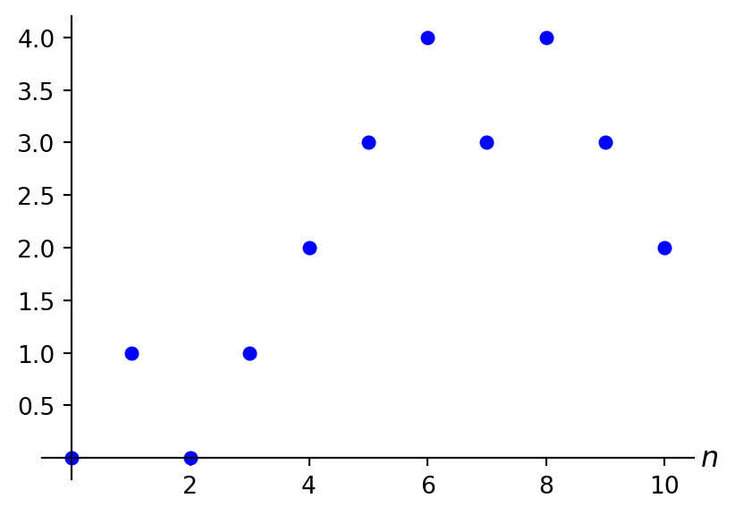
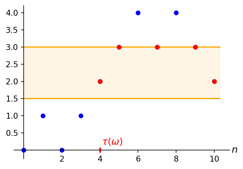
Let $\tau$ be the first hitting time of $B$ i.e. the first time $n$ for which $X_n \in B$. That is: \[\tau(\omega):=\inf \{ n=0,1,\ldots \, | \, X_n(\omega) \in B\} \quad \text{for all } \omega \in \Omega.\] Make sure to read this correctly: for any $\omega \in \Omega$, we consider \[\{ n=0,1,\ldots \, | \, X_n(\omega) \in B\}\] i.e. the set of time points $n$ for which $X_n(\omega) \in B$ and then we take the infimum of this set (see Wiki if you’d like a reminder). If this set contains one or more time points, then its infimum is simply the smallest of these i.e. the first time that the path of the process we’re considering hits/enters the set $B$. If this set is empty (because the path of the process we’re considering never hits/enters $B$) then we end up with $\inf \emptyset$ and by convention we have/define $\inf \emptyset:=\infty$. So we see that \[\tau(\omega) \in \{0,1,\ldots\} \cup \{\infty\},\] with $\tau(\omega)=\infty$ if and only if $X_n(\omega) \in B^c$ for all $n=0,1,\ldots$.

If the story we told in this section was clear to you, then you should be able to convince yourself intuitively pretty quickly that this is indeed a stopping time: as you follow a path of the process through time, at any time $n$ you can decide whether or not this is your $\tau(\omega)$ only using $X_0(\omega), \ldots, X_n(\omega)$ — indeed your decision is positive if and only if $X_n(\omega) \in B$ while $X_0(\omega), \ldots, X_{n-1}(\omega) \in B^c$. It is often quite useful to use such intuition to quite quickly convince yourself whether or not a given candidate is indeed a stopping time (before confirming — or maybe not! — by a mathematical argument as needs be, but then also the way you set up the mathematical argument is typically strongly influenced by this intuition)!

It’s not hard to verify from Definition 6.1 that $\tau$ is indeed a stopping time: for any $n=0,1,\ldots$, $\tau(\omega) \leq n$ if and only if at least one of $X_0(\omega), \ldots, X_n(\omega)$ is an element of $B$, that is \[\{ \tau \leq n \} = \bigcup_{i=0}^n \{ X_i \in B \}. \tag{6.4}\] Since $(X_n)_{n=0,1,\ldots}$ is adapted, for each $i=0,\ldots,n$ we have that $X_i$ is $\mathcal{F}_i$-measurable and hence $\mathcal{F}_n$-measurable (non-decreasing property of filtrations again). This means by def (cf. Definition 2.1) that $\{ X_i \in B \} \in \mathcal{F}_n$, and from Definition 1.1 also Equation 6.4 is an element of $\mathcal{F}_n$.

Note: we could of course also have argued via events $\{ \tau = n \}$ rather, which is maybe a bit more natural from the intuition — it’s just that this argument is a bit more convenient for when we consider stopping times in continuous time later on.

See Figure 6.1 for a visualisation.

(a) A path (well at least the first part of it) $X_0(\omega), X_1(\omega), \ldots$ of a process $(X_n)_{n=0,1,\ldots}$ in our favourite visualisation stemming from Figure 5.1 (b)

Exercises

You can now do Exercise 6.1–Exercise 6.2.

6.3 Stopped processes & martingales

Naturally with the concept of stopping times as just discussed, comes the concept of a stopped process: consider an adapted process $(X_n)_{n=0,1,\ldots}$ on some filtered probability space $(\Omega,\mathcal{F},(\mathcal{F}_n)_{n=0,1,\ldots},\P)$ and let $\tau$ be stopping time on this space as just defined in Definition 6.1. Now imagine that you create a new process as follows: for any $\omega \in \Omega$, you let the corresponding path of $(X_n)_{n=0,1,\ldots}$ evolve as normal but only until you reach the time point $\tau(\omega)$, from then onwards you keep the path fixed at that value forever. Indeed this is quite literally an act of “stopping” the process, and this also explains a bit more clearly why we used the term “stopping time” in the previous section! See Figure 6.2 for a visual.

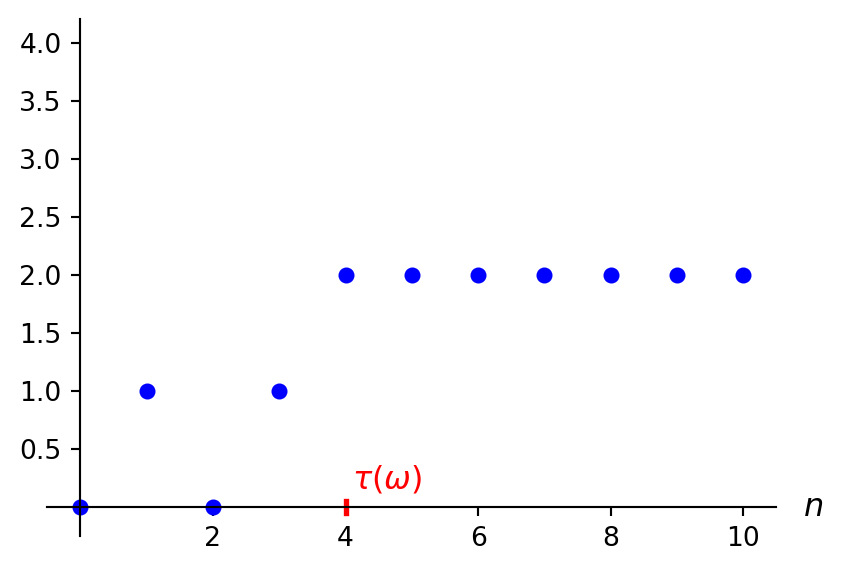
Figure 6.2: Considering again the path of the process $(X_n)_{n=0,1,\ldots}$ and the stopping time $\tau$ from Figure 6.1, with $\tau(\omega)=4$ for the path in question, this is what the corresponding path of the *stopped* process looks like

In terms of maths, we denote this modification of $(X_n)_{n=0,1,\ldots}$ by stopping it at time $\tau$ by² $(X^\tau_n)_{n=0,1,\ldots}$, and we could write down an expression as follows: \[X^\tau_n = X_{n \wedge \tau} = \mathbf{1}_{\{ n < \tau\}} X_n + \mathbf{1}_{\{ n \geq \tau\}} X_\tau \quad \text{for all } n=0,1,\ldots, \tag{6.5}\] where “$n \wedge \tau$” is common shorthand for “$\min\{n,\tau\}$”. Note that these two indicator functions act as “switches” if you will: always exactly one of these two is equal to $1$ (and the other equal to $0$), depending on whether on the time axis we are in $\{0,\ldots,\tau-1\}$ where the path evolves as normal or we are in $\{\tau,\tau+1,\tau+2,\ldots\}$ where the path is kept constant at value $X_\tau$.

² Note that the “${}^\tau$” in “$X^\tau_n$” is just for decoration, it is not a power or so and neither can you plug an $\omega$ into that particular $\tau$, it’s only there to signal a stopped process

Indeed, if we plug in an $\omega \in \Omega$ (obviously we need to do this both in each $X_n$ as well as in $\tau$ as these are all mappings/random variables), then this works out to (using a case distinction rather than indicator functions as we did in Equation 6.5) \[X^\tau_n(\omega)=X_{n \wedge \tau(\omega)}(\omega)= \begin{cases} X_n(\omega) & \text{if $n \leq \tau(\omega)$} \\ X_{\tau(\omega)}(\omega) & \text{if $n > \tau(\omega)$} \end{cases} \quad \text{for all } n=0,1,\ldots, \tag{6.6}\] which hopefully convinces you that indeed these expressions represent the idea from the first paragraph. (To recreate the example path in Figure 6.2, you’d plug in $\tau(\omega)=4$ — convince yourself that with this choice Equation 6.6 exactly generates Figure 6.2!) Observe that if $\tau(\omega)=\infty$, then the “stopping” never happens and hence the path of the stopped process is just the same as the path of the original process, note that indeed Equation 6.5 and Equation 6.6 respect this as well.

There are two properties we want to investigate in this section: whether or not a stopped process is also adapted (to the same filtration as the original process), and whether stopping a (sub/super)martingale again results in a (sub/super)martingale.

To study stopped processes and to answer these questions, the formulation using indicator functions as used in Equation 6.5 is often quite useful. Indeed let’s look at the stopped process being adaptable first, i.e. to show that for each $n=0,1,\ldots$, $X^\tau_n$ is $\mathcal{F}_n$-measurable. As we mentioned in Example 6.1 as well, it is always good to first check your intuition: do you believe that $X^\tau_n$ is $\mathcal{F}_n$-measurable i.e. more intuitively speaking, that at time $n$ you have enough information to deduce what value $X^\tau_n$ has? Well yes: we follow the path as normal up until time $\tau(\omega)$ so that’s covered by the fact that the (original) process is adapted, and once we decide to stop we do that based on information available at that point in time (by def of a stopping time), and after that stopping point we know that stopping has happened in the past and at what value. So at no point do we use any information “from the future”. Note that it is important here how stopping times are defined — indeed the “measurability constraints” we imposed there are (also) to make sure that the stopped process remains adapated!

Ok, let’s try to actually prove this. Fix some $n=0,1,\ldots$ and we set out to prove that $X^\tau_n$ is $\mathcal{F}_n$-measurable. Recall from Exercise 6.1 that $\{ n < \tau\}=\{\tau>n\} \in \mathcal{F}_n$ from which it follows that $\mathbf{1}_{\{ n < \tau\}}$ is $\mathcal{F}_n$-measurable (cf. Exercise 2.3). Since $X_n$ is also $\mathcal{F}_n$-measurable (the process is adapted), also the product $\mathbf{1}_{\{ n < \tau\}} X_n$ is $\mathcal{F}_n$-measurable (cf. Proposition 2.1 iv e.g.). For the second term in Equation 6.5 you could for instance write \[\begin{aligned} \mathbf{1}_{\{ n \geq \tau\}} X_\tau &= \mathbf{1}_{\{ \tau \leq n\}} X_\tau \\ &= \sum_{i=0}^n \mathbf{1}_{\{ \tau =i\}} X_\tau \\ &= \sum_{i=0}^n \mathbf{1}_{\{ \tau =i\}} X_i, \end{aligned} \tag{6.7}\] where for the second equality we used that since $\{ \tau =0\}$, $\{ \tau =1\}$, …, $\{ \tau =n\}$ forms a partition (cf. Section 1.2.3) of the event $\{\tau \leq n\}$, a slight extension of Exercise 4.2 shows that we can write the indicator function as a sum of indicator functions; and the final equality is essentially a tautology: for any $\omega \in \Omega$ \[\begin{aligned} \mathbf{1}_{\{ \tau =i\}}(\omega) X_{\tau(\omega)}(\omega) &= \begin{cases} X_{\tau(\omega)}(\omega) & \text{if $\tau(\omega)=i$} \\ 0 & \text{otherwise} \end{cases} \\ &= \begin{cases} X_{i}(\omega) & \text{if $\tau(\omega)=i$} \\ 0 & \text{otherwise} \end{cases} \\ &= \mathbf{1}_{\{ \tau =i\}}(\omega) X_i(\omega). \end{aligned} \] Now, since by def of a stopping time (cf. Definition 6.1) $\{ \tau =i\} \in \mathcal{F}_i \subseteq \mathcal{F}_n$, similar arguments as above show that the ultimate right hand side in Equation 6.7 is $\mathcal{F}_n$-measurable and hence so is the ultimate left hand side. Overall, we have now shown that both terms in the right hand side of Equation 6.5 are $\mathcal{F}_n$-measurable and hence so is $X^\tau_n$.

The second property we wanted to investigate is whether a (sub/super)martingale is preserved — the answer is “yes” and we leave the proof of this one for Exercise 6.4.

Proposition 6.1 On some filtered probability space $(\Omega,\mathcal{F},(\mathcal{F}_n)_{n=0,1,\ldots},\P)$, let $(X_n)_{n=0,1,\ldots}$ be an adapted process and let $\tau$ be a stopping time (cf. Definition 6.1) on this space. Then the corresponding stopped process $(X^\tau_n)_{n=0,1,\ldots}$ consists of random variables defined as follows: \[X^\tau_n = X_{n \wedge \tau} = \mathbf{1}_{\{ n < \tau\}} X_n + \mathbf{1}_{\{ n \geq \tau\}} X_\tau \quad \text{for all } n=0,1,\ldots,\] where “$n \wedge \tau$” is common shorthand for “$\min\{n,\tau\}$”. It has the following properties.

$(X^\tau_n)_{n=0,1,\ldots}$ is adapted.
If $(X_n)_{n=0,1,\ldots}$ is a (sub/super)martingale, then $(X^\tau_n)_{n=0,1,\ldots}$ is also a (sub/super)martingale.

Exercises

You can now do Exercise 6.3–Exercise 6.4.

6.4 Doob’s (& Hunt’s) optional stopping theorem

The optional stopping theorems build on the concept of stopping times and stopped processes, and state a result that is on the one hand kind of obviuous (or at least not very unexpected), but that nevertheless turn out to be very consequential — we’ll see some of that in Chapter 7!

The starting point is a filtered probability space $(\Omega,\mathcal{F},(\mathcal{F}_n)_{n=0,1,\ldots},\P)$ on which an adapted process $(X_n)_{n=0,1,\ldots}$ and a stopping time $\tau$ live. Recall from Definition 6.1 that in principle $\tau$ can take the value $\infty$, in this setting we assume that this does not happen almost surely i.e. that $\P(\tau<\infty)=1$ (however see Remark 6.2).

Out of these ingredients we can create a new random variable as follows: for each $\omega \in \Omega$, take from the path $X_0(\omega), X_1(\omega), \ldots$ the value at which you stop the process i.e. $X_{\tau(\omega)}(\omega) \in \R$. This clearly creates a mapping $X_\tau: \Omega \to \R$, at least for those $\omega \in \Omega$ for which $\tau(\omega)<\infty$. Under our standing assumption that $\tau<\infty$ a.s. (only), this may mean that we have to leave $X_\tau$ undefined (or give it some arbitrary value, e.g. $0$) on the event $\{\tau=\infty\}$ — but we have encountered such a contsruction a few times now so hopefully it doesn’t scare you too much anymore! To see that $X_\tau$ is $\mathcal{F}$-measurable and hence indeed a random variable, you can for instance write (using the same arguments as for Equation 6.7, and ignoring what happens on the event $\{\tau=\infty\}$ if indeed not empty) \[X_\tau = \sum_{i=0}^\infty \mathbf{1}_{\{\tau=i\}} X_i \tag{6.8}\] and observe that since every term in the sum is $\mathcal{F}$-measurable, so is the sum (cf. Proposition 2.1)³.

³ If you don’t find this entirely satisfactory, note that for each $\omega$, only a single term in this infinite sum is non-zero so convergence of the partial sums to the infinite sum is trivial

Here’s the point: recall that if $(X_n)_{n=0,1,\ldots}$ is a martingale then it has constant expectations i.e. $\E[X_n]=\E[X_0]$ for all $n=0,1,\ldots$ (cf. Equation 5.11). This new random variable $X_\tau$ is, loosely speaking, a mix of values from $X_0, X_1, \ldots$ stirred (not shaken) together by the random timepoint $\tau$. So it is natural to wonder whether this constant expectations property extends to $X_\tau$ as well i.e. whether \[\E[X_\tau]=\E[X_0]. \tag{6.9}\] Indeed that turns out to be true, provided things aren’t too crazy.

First consider the case that $\tau$ is a.s. bounded, i.e. that an $N \in \{0,1,\ldots\}$ exists so that $\P(\tau \leq N)=1$. In this case we can simply use Proposition 6.1: the stopped process $(X^\tau_n)_{n=0,1,\ldots}$ is (also) a martingale and hence also has the property of constant expectations (note that trivially $0 \wedge \tau=0$): \[\E[X_{n \wedge \tau}]=\E[X_0] \quad \text{for all } n=0,1,\ldots. \tag{6.10}\] If we now choose any $n \geq N$, then since $\tau \leq N \leq n$ a.s., $n \wedge \tau=\tau$ a.s. and hence also $X_{n \wedge \tau}=X_\tau$ a.s. Since expectations don’t care about a.s. differences (cf. Proposition 3.6 ii), it follows from Equation 6.10 that also Equation 6.9 holds.

Now consider the case that $\tau$ is not necessarily any longer a.s. bounded (but we do keep the assumption that $\tau<\infty$ a.s. in force). Looking again at Equation 6.10, how could we (now) get to Equation 6.9? Well indeed, it is quite tempting to take the limit for $n \to \infty$ in Equation 6.10! Clearly, fixing any $\omega \in \{\tau<\infty\}$, for all $n>\tau(\omega)$ we have that $n \wedge \tau(\omega)=\tau(\omega)$ and hence also \[X_{n \wedge \tau(\omega)}(\omega)=X_{\tau(\omega)}(\omega).\] Hence (trivially) $X_{n \wedge \tau(\omega)}(\omega)$ converges to $X_{\tau(\omega)}(\omega)$ as $n \to \infty$. This shows that \[X_{n \wedge \tau} \stackrel{\text{a.s.}}{\longrightarrow} X_{\tau} \quad \text{as $n \to \infty$} \tag{6.11}\] (almost surely only because we ignore $\omega \in \{\tau=\infty\}$ for which we haven’t properly defined $X_\tau$). So, if it follows from Equation 6.11 that also their expectations converge i.e. \[\lim_{n \to \infty} \E[X_{n \wedge \tau}]=\E[X_{\tau}], \tag{6.12}\] then Equation 6.10 implies that Equation 6.9 follows as well!

So the final piece of the puzzle is: under what condition (if any) does it hold that the a.s. convergence from Equation 6.11 implies convergence of the corresponding expectations i.e. Equation 6.12? Maybe the bell is already ringing with you: we have seen two results dealing with this, namely the MCT and the DCT (cf. Section 3.5). The MCT does not (necessarily) apply here (in general we won’t have the required monotonicity etc.) so the honours go to the DCT. This brings us to our first optional stopping theorem:

Theorem 6.1 (Doob’s optional stopping theorem) On some filtered probability space $(\Omega,\mathcal{F},(\mathcal{F}_n)_{n=0,1,\ldots},\P)$, let $(X_n)_{n=0,1,\ldots}$ be a martingale and $\tau$ a stopping time with the property that $\tau<\infty$ a.s.

Then $X_\tau$ is a random variable, and if one of the following two conditions holds:

$\tau$ is a.s. bounded (i.e. there exists an $N=0,1,\ldots$ so that $\P(\tau \leq N)=1$),
there exists an integrable random variable $Y$ so that $\lvert X_{n \wedge \tau} \rvert \leq Y$ a.s. for all $n=0,1,\ldots$,

then we have that $\E[X_\tau]=\E[X_0]$.

This results remains valid if $(X_n)_{n=0,1,\ldots}$ is a sub- resp. supermartingale, in which case the conclusion is $\E[X_\tau] \geq \E[X_0]$ resp. $\E[X_\tau] \leq \E[X_0]$ (of course, still provided that one of the conditions i or ii holds).

Example 6.2 This example also serves as a serious warning! In our discussion so far we have seen (and I hope that you agree) that the result from Doob’s optional stopping theorem makes a lot of sense, and it may be tempting to think that the result will be true in general i.e. that the conditions in Theorem 6.1 are actually not necessary.

However this is not the case! Indeed consider for instance the accumulated profit process $(X_n)_{n=0,1,\ldots}$ from playing the same game repeatedly (and independently) from Example 5.3. Recall that we start with a profit of $0$ i.e. $X_0=0$ and we had also seen that if we assume the expected profit per game, $\E[Y]$, to equal $0$ then $(X_n)_{n=0,1,\ldots}$ is a martingale.

Now consider the following stopping time: \[\tau=\inf \{ n=0,1,\ldots \, | \, X_n \geq 10 \}\] i.e. the first hitting time of the interval $[10,\infty)$ as discussed in Example 6.1 (which we’ve also verified in that example to indeed be a stopping time). It is not entirely obvious but it can be shown that $\tau<\infty$ a.s. — not entirely obvious because there will indeed be paths of the process that never reach the level $10$ at all, just imagine that you have a very unlucky evening and lose a lot of the games that you play, but it can be shown that such paths make up an event of probability $0$ only.

Observe that when $\tau<\infty$, then at time $\tau$, by def your accumulated profit is at least equal to $10$ i.e. $X_\tau \geq 10$. So $X_\tau \geq 10$ a.s. and hence $\E[X_\tau] \geq 10$ (cf. Proposition 3.6 ii). Yet since $X_0=0$ also $\E[X_0]=0$ and hence we have that \[\E[X_\tau] \not= \E[X_0] \quad \text{!}\]

So apparently the conclusion from Theorem 6.1 does not apply in this example, meaning that also neither of the conditions i and ii in the theorem hold. It’s not hard to imagine that $\tau$ does not satisfy the boundedness from condition i — basically because you can keep experiencing losing streaks it can take an arbitrarily long time to reach an accumulated profit of $10$. For condition ii, apparently there does not exist an integrable $Y$ that satisfies $\lvert X_{n \wedge \tau} \rvert \leq Y$ a.s. for all $n=0,1,\ldots$. The reason is that even though the accumulated profit can’t get too large (after all, as soon as it exceeds $10$ we stop and stay stuck at the level we’re at), we also have to take into account negative accumulated profits and there is no control on those. Obviously the absolute value ensures that (very) large negative values for $X_{n \wedge \tau}$ result in (very) large positive values for $\lvert X_{n \wedge \tau} \rvert$. And apparently that aspect is significant enough that it causes there not to exist an integrable upperbound on $\lvert X_{n \wedge \tau} \rvert$!

In addition to Doob’s optional stopping theorem, in which we compare $\E[X_\tau]$ with $\E[X_0]$, if we have two stopping times, say $\sigma$ and $\tau$ with $\sigma \leq \tau$ (a.s.), then we might want to compare $\E[X_\sigma]$ with $\E[X_\tau]$ as well. Note that if $(X_n)_{n=0,1,\ldots}$ is a martingale and if both stopping times are bounded, then it follows from Doob’s optional stopping theorem that \[\E[X_\tau]=\E[X_0]=\E[X_\sigma]\] i.e. that $\E[X_\sigma]$ and $\E[X_\tau]$ are equal as you’d probably expect from the constant expectation property of martingales. On the other hand, if $(X_n)_{n=0,1,\ldots}$ is a supermartingale then its expectations are non-increasing with $n$ (recall from Equation 5.13) then since $\sigma \leq \tau$ it makes sense that this would yield $\E[X_\sigma] \geq \E[X_\tau]$. This is cofirmed, at least for bounded stopping times, in the following result with which we wrap up this section:

Theorem 6.2 (Hunt’s optional stopping theorem) On some filtered probability space $(\Omega,\mathcal{F},(\mathcal{F}_n)_{n=0,1,\ldots},\P)$, let $(X_n)_{n=0,1,\ldots}$ be a supermartingale and let $\sigma, \tau$ be two stopping times on this space with the following two properties:

$\sigma \leq \tau$ (a.s.),
$\tau$ is a.s.bounded (with the same meaning as in Theorem 6.1 condition i).

Then we have that $\E[X_\sigma] \geq \E[X_\tau]$.

If $(X_n)_{n=0,1,\ldots}$ is a martingale resp. submartingale, then the conclusion is $\E[X_\sigma] = \E[X_\tau]$ resp. $\E[X_\sigma] \leq \E[X_\tau]$ rather (under the same conditions on the stopping times obviously).

Proof. It is enough to prove the supermartingale statement, because if $(X_n)_{n=0,1,\ldots}$ is a submartingale then we can apply the supermartingale statement to $(-X_n)_{n=0,1,\ldots}$ and if $(X_n)_{n=0,1,\ldots}$ is a martingale then we can use that it is both a sub- and supermartingale (or use Doob’s optional stopping theorem as mentioned above).

So let $(X_n)_{n=0,1,\ldots}$ be a supermartingale. Also it is enough to consider only those $\omega \in \Omega$ for which $0 \leq \sigma(\omega) \leq \tau(\omega) \leq N$ (where $N=0,1,\ldots$ is the constant that comes from the assumption that $\tau$ is bounded) since they make up an event of probahblity $1$ which is enough to prove the conclusion since expectations don’t care about probability $0$ events (and neither will other steps in the proof below).

Now, the supermartingale property tells us how $X_{n+1}$ relates to $X_n$ (cf. Equation 5.10) and the idea is to use that to connect $X_{\sigma}$ with $X_\tau$. However the problem is of course that for different $\omega$, $\sigma(\omega)$ and $\tau(\omega)$ can be in very different places on the time axis so we need to be careful to get this right. First note that for any $\omega$, we can use the idea of a telescoping sum to (trivially!) connect $X_{\sigma(\omega)}(\omega)$ with $X_{\tau(\omega)}(\omega)$ as follows: \[\begin{aligned} & X_{\tau(\omega)}(\omega)-X_{\sigma(\omega)}(\omega) = \sum_{n=\sigma(\omega)}^{\tau(\omega)-1} (X_{n+1}(\omega)-X_n(\omega)) \implies \\ & X_{\tau(\omega)}(\omega) = X_{\sigma(\omega)}(\omega) + \sum_{n=\sigma(\omega)}^{\tau(\omega)-1} (X_{n+1}(\omega)-X_n(\omega)). \end{aligned} \] So now we do have a sum of increments $X_{n+1}-X_n$, but since $\omega$ appears in the bounds of the sum we can’t do much with it yet. The key trick is to bring that dependence into the sum by means of an indicator function: \[X_{\tau(\omega)}(\omega) = X_{\sigma(\omega)}(\omega) + \sum_{n=0}^N \mathbf{1}_{\{ \sigma \leq n < \tau \}}(\omega) (X_{n+1}(\omega)-X_n(\omega)),\] indeed note that this indicator function makes sure that in this sum, only the terms that we actually want to keep are multiplied by $1$ and all others vanish since they get multiplied by $0$. Also note that the upperbound $N$ is large enough due to $0 \leq \sigma(\omega) \leq \tau(\omega) \leq N$. So now we can write this as an identity between mappings: \[X_{\tau} = X_{\sigma} + \sum_{n=0}^N \mathbf{1}_{\{ \sigma \leq n < \tau \}} (X_{n+1}-X_n).\]

Now, taking expectations on both sides of this identity, we see that the result follows provided we can show that \[\E \big[ \mathbf{1}_{\{ \sigma \leq n < \tau \}} (X_{n+1}-X_n) \big] \leq 0 \quad \text{for all $n=0,1,\ldots$.} \tag{6.13}\] Recall that the supermartingale property Equation 5.10 allows us to deal with the difference $X_{n+1}-X_n$ conditional on $\mathcal{F}_n$. But that indicator function… However, if we could show that it is $\mathcal{F}_n$-measurable, then by the “taking out what is known” rule for conditional expectations we could, indeed, take it out of the conditional expectation and properly make use of the supermartingale property! Indeed this works.

First for that indicator. Note that for any $n=0,1,\ldots$ \[\{ \sigma \leq n < \tau \} = \{ \sigma \leq n\} \cap \{\tau>n \}\] and since both events on the right hand side are elements of $\mathcal{F}_n$ (the first one by def, cf. Definition 6.1, and the second by Exercise 6.1) also their intersection and hence the left hand side is an element of $\mathcal{F}_n$ (cf. Proposition 1.1). This implies that $\mathbf{1}_{\{ \sigma \leq n < \tau \}}$ is $\mathcal{F}_n$-measurable (cf. Exercise 2.3).

Now we can wrap up the proof as laid out above: \[\begin{aligned} \E \big[ \mathbf{1}_{\{ \sigma \leq n < \tau \}} (X_{n+1}-X_n) \big] &= \E \big[ \E \big[ \mathbf{1}_{\{ \sigma \leq n < \tau \}} (X_{n+1}-X_n) \, \big| \, \mathcal{F}_n \big] \big] \\ &= \E \big[ \mathbf{1}_{\{ \sigma \leq n < \tau \}} \E \big[ (X_{n+1}-X_n) \, \big| \, \mathcal{F}_n \big] \big] \\ &\leq 0, \end{aligned} \] confirming that Equation 6.13 indeed holds. For the first equality we used Theorem 4.2 i, for the second Theorem 4.2 v, and for the inequality we used that $\E [ (X_{n+1}-X_n) \, | \, \mathcal{F}_n ] \leq 0$ a.s. (the supermartingale property), multiplying by the non-negative indicator function keeps it $\leq 0$ a.s., plus non-negativity of expectations (cf. Proposition 3.6 ii).

Remark 6.2. We have formulated the optional stopping results in this section only for stopping times that are finite almost surely, because (for starters) it’s not even clear what $X_\tau$ should mean if $\tau$ is not finite. But actually, we do know something about this — indeed Doob’s martingale convergence theorem (cf. Theorem 5.2) tells us that under some conditions, the process has an a.s. limit as $n \to \infty$. Would it then not make sense to understand/define $X_\tau$ to be equal to this limit if $\tau=\infty$? And could we somehow still make the optional stopping results above work if we allow for this? The answer is generally “yes” — but unfortunately we don’t really have the time to pursue this properly.

Exercises

You can now do Exercise 6.5–Exercise 6.7.

6.5 Doob’s maximal inequalities

We conclude this chapter by exploring some more properties of martingales, this time we are particularly interested in how large the values of a martingale can get. As an advance warning: some of the proofs that we’ll encounter are a bit technical. Please don’t let that discourage you — I’ve tried to write them out in much detail to hopefully make them clear to you. On the one hand, don’t ignore them and try to understand them, especially if you want to pursue a career in a high level maths environment (be it in academia or industry) there is a lot of tools for your toolbox to pick up! On the other hand, of course please don’t worry that the exam will ask you to regurgitate, let alone invent on the spot, such a long/technically demanding proof.

To discuss the direction of thinking, let’s first write down the following little

Lemma 6.1 Let $(X_n)_{n=0,1,\ldots}$ be a martingale on some filtered probability space $(\Omega,\mathcal{F},(\mathcal{F}_n)_{n=0,1,\ldots},\P)$ and fix some $n=0,1,\ldots$. Then \[X_k=\E[X_n \, | \, \mathcal{F}_k] \quad \text{for all } k=0,\ldots,n. \tag{6.14}\]

Proof. Note that for $k=n$ this is trivial ($X_n$ is $\mathcal{F}_n$-measurable and Theorem 4.2 ii kicks in), for $k=n-1$ this is nothing but the martingale property (cf. Equation 5.8), but indeed it holds for smaller values of $k$ as well.

To see this, we first use the same trick as in the proof of Theorem 6.2 namely a telescoping sum to write $X_n-X_k$ as a sum of differences over one time step only, and then apply the martingale property to each of these one time step differences. That is, we write \[X_n-X_k = \sum_{i=k}^{n-1} (X_{i+1}-X_i)\] so that by linearity of conditional expectations \[\E[X_n - X_k \, | \, \mathcal{F}_k]=\sum_{i=k}^{n-1} \E[X_{i+1} - X_i \, | \, \mathcal{F}_k]\] and hence Equation 6.14 follows if we can show that for any $i=k,\ldots,n-1$ it holds that \[\E[X_{i+1} - X_i \, | \, \mathcal{F}_k]=0.\] This is almost the martingale property (in the formulation of Exercise 5.3), except to apply that one we’d need to be conditioning on $\mathcal{F}_i$ rather than $\mathcal{F}_k$. For “switching” from conditioning on one $\sigma$-algebra to another one we have the perfect tool: the tower property (cf. Theorem 4.2 iv)! Indeed, since $i \geq k$ we also have $\mathcal{F}_k \subseteq \mathcal{F}_i$ (since a filtration is non-decreasing, cf. Definition 5.1) and hence by the tower property \[\E[X_{i+1} - X_i \, | \, \mathcal{F}_k] = \E \big[ \E[X_{i+1} - X_i \, | \, \mathcal{F}_i] \, \big| \, \mathcal{F}_k \big]=\E[0 \, | \, \mathcal{F}_k]=0.\]

What Equation 6.14 is shouting at us: for any $n$, all the earlier random variables $X_0,\ldots,X_{n-1}$ are determined by $X_n$. So it makes some sense to hope that we can control how large any of the $X_0,\ldots,X_{n-1}$ can get by controlling how large $X_n$ can get. And indeed your new friend Doob is delivering here as well!

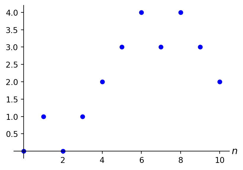
To control the size of a bunch of random variables simultaneously, it is natural to look at the maximum of their (absolute) values. Therefore we introduce, for any given process $(X_n)_{n=0,1,\ldots}$, its running maximum(/supremum) process denoted by $(X^*_n)_{n=0,1,\ldots}$ and defined as \[X^*_n := \max_{k=0,\ldots,n} \lvert X_k \rvert \quad \text{for all } n=0,1,\ldots. \tag{6.15}\] Note the absolute value, ensuring that both large positive and large negative values among $X_0,\ldots,X_n$ translate to a large (positive) value for $X^*_n$. Observe that what Equation 6.15 means is that for any $\omega \in \Omega$, the path of $(X^*_n)_{n=0,1,\ldots}$ is determined from the path of $(X_n)_{n=0,1,\ldots}$ by means of \[\begin{aligned} & X^*_0(\omega) = \lvert X_0(\omega) \rvert, \quad X^*_1(\omega)=\max \{ \lvert X_0(\omega) \rvert, \lvert X_1(\omega) \rvert \}, \\ & X^*_2(\omega) =\max \{ \lvert X_0(\omega) \rvert, \lvert X_1(\omega) \rvert, \lvert X_2(\omega) \rvert \}, \quad \ldots. \end{aligned} \] In particular, $(X^*_n)_{n=0,1,\ldots}$ is a non-negative process with non-decreasing paths, and it is adapted if $(X_n)_{n=0,1,\ldots}$ is. It is also useful to be aware of the following alternative definition/formulation in recursive form: \[X^*_0=\lvert X_0 \rvert, \quad X^*_n = \max \{ X^*_{n-1}, \lvert X_n \rvert \} \quad \text{for all } n=1,2,\ldots. \tag{6.16}\] Figure 6.3 gives a visual — convince yourself that you understand how the path in Figure 6.3 (b) follows from the one in Figure 6.3 (a)!

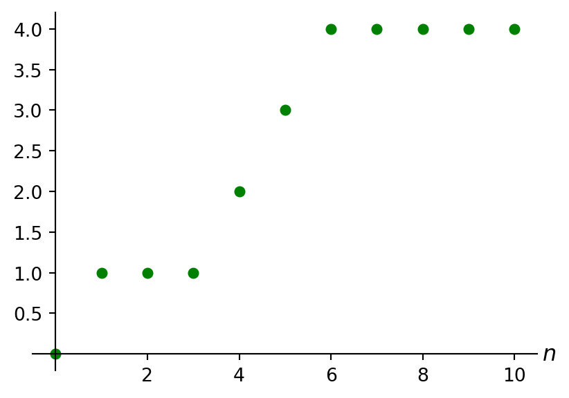
Withour further ado, here is the theorem of this section — two again very useful and important results, devoted to bounding $X^*_n$ in terms of $X_n$:

Theorem 6.3 (Doob’s martingale inequalities) On some filtered probability space $(\Omega,\mathcal{F},(\mathcal{F}_n)_{n=0,1,\ldots},\P)$, let $(X_n)_{n=0,1,\ldots}$ be one of the following:

a martingale,
a non-negative submartingale,
a non-positive supermartingale.

Further let $(X^*_n)_{n=0,1,\ldots}$ be its running maximum process as defined in Equation 6.15 and/or Equation 6.16.

Fix some $n=0,1,\ldots$. We have the following:

Maximal inequality: for any $\lambda >0$, \[\lambda \P(X^*_n \geq \lambda) \leq \E[\mathbf{1}_{\{X^*_n \geq \lambda\}} \lvert X_n \rvert] \leq \E[\lvert X_n \rvert].\]
$L^p$-inequality: for any $p>1$: \[\E[(X^*_n)^p] \leq \left( \frac{p}{p-1} \right)^p \E[\lvert X_n \rvert^p].\]

Note that in i, the right hand side is guaranteed to be finite (because $(X_n)_{n=0,1,\ldots}$ is integrable by assumption), while in ii both the left and right hand side could be infinite for some or even all $p>1$. This doesn’t make the $L^p$-inequality any less true of course, but obviously the right hand side doesn’t make for a very useful upperbound if it’s infinite!

Proof. Consider the “absolute value” process $(Y_n)_{n=0,1,\ldots}$ given by $Y_n=\lvert X_n \rvert$. This process is obviously non-negative and also a submartingale (cf. Exercise 6.8).

For part i, fix some $n=0,1,\ldots$. Consider the mapping \[\tau = \inf \{ k=0,1,\ldots \, | \, Y_k \geq \lambda \} \wedge n \tag{6.17}\] (recall from Section 6.3 that “$a \wedge b$” is shorthand for “$\min\{a,b\}$”). Since a fixed time is trivially a stopping time, it follows from Example 6.1 and Exercise 6.2 that $\tau$ is also a stopping time. Applying Hunt’s optional stopping theorem Theorem 6.2 with $\tau$ and $n$ as stopping times we get that \[\E[Y_\tau] \leq \E[Y_n]. \tag{6.18}\] Now note that \[\E[Y_\tau] = \E \big[ \big( \mathbf{1}_{\{Y^*_n<\lambda\}}+\mathbf{1}_{\{Y^*_n \geq \lambda\}} \big) Y_\tau \big] = \E \big[ \mathbf{1}_{\{Y^*_n<\lambda\}} Y_\tau \big] + \E \big[ \mathbf{1}_{\{Y^*_n \geq \lambda\}} Y_\tau \big]. \tag{6.19}\] We do some work on both terms in the ultimate right hand side separately.

First, if $\omega \in \{Y^*_n<\lambda\}$ i.e. $Y^*_n(\omega)<\lambda$, then by def of the running max process (cf. Equation 6.15) $Y_i(\omega)<\lambda$ for all $i=0,\ldots,n$ so that $\tau(\omega) =n$ (by def, cf. Equation 6.17) and $Y_{\tau(\omega)}(\omega)=Y_n(\omega)$. This yields \[\E \big[ \mathbf{1}_{\{Y^*_n<\lambda\}} Y_\tau \big] = \E \big[ \mathbf{1}_{\{Y^*_n<\lambda\}} Y_n \big].\]

Secondly, if $\omega \in \{Y^*_n \geq \lambda\}$ i.e. $Y^*_n(\omega) \geq \lambda$, then again by def of the running max process, there exists an $i \in \{0,\ldots,n\}$ so that $Y_i(\omega) \geq \lambda$ and hence (by def, cf. Equation 6.17) $\tau(\omega)$ is the smallest of such $i$’s with in particular $Y_{\tau(\omega)}(\omega) \geq \lambda$. This hence yields \[\E \big[ \mathbf{1}_{\{Y^*_n \geq \lambda\}} Y_\tau \big] \geq \E \big[ \mathbf{1}_{\{Y^*_n\geq \lambda\}} \lambda \big]=\lambda \E \big[ \mathbf{1}_{\{Y^*_n \geq \lambda\}} \lambda \big] = \lambda \P(Y^*_n \geq \lambda).\]

Now plugging these two considerations into Equation 6.19 gives us \[\E[Y_\tau] \geq \lambda \P(Y^*_n \geq \lambda) + \E \big[ \mathbf{1}_{\{Y^*_n<\lambda\}} Y_n \big]\] and then going back to Equation 6.18 we see that \[\E[Y_n] \geq \lambda \P(Y^*_n \geq \lambda) + \E \big[ \mathbf{1}_{\{Y^*_n<\lambda\}} Y_n \big]\] i.e. \[\lambda \P(Y^*_n \geq \lambda) \leq \E[Y_n]-\E \big[ \mathbf{1}_{\{Y^*_n<\lambda\}} Y_n \big] = \E \big[ \mathbf{1}_{\{Y^*_n \geq \lambda\}} Y_n \big]\] and since $Y_n \geq 0$, this ultimate right hand side is also bounded above by $\E[Y_n]$.

Now just sub $\lvert X_n \rvert$ back in for $Y_n$, and observe that (trivially) $Y^*_n=X^*_n$ to arrive at the result as stated.

For part ii, again fix some $n=0,1,\ldots$ and also some $K=1,2,\ldots$. Then we can argue as follows: \[\begin{aligned} \E[(Y^*_n \wedge K)^p] &= \int_0^K pt^{p-1} \P(Y^*_n>t) \d t \\ &= \int_0^K pt^{p-2} t \P(Y^*_n>t) \d t \\ &\leq \int_0^K pt^{p-2} \E[\mathbf{1}_{\{Y^*_n \geq t\}} Y_n] \d t \\ &= \E \left[ Y_n \int_0^K pt^{p-2} \mathbf{1}_{\{Y^*_n \geq t\}} \d t \right] \\ &= \E \left[ Y_n \int_0^{Y^*_n \wedge K} pt^{p-2} \d t \right] \\ &= \E \left[ Y_n \frac{p}{p-1} (Y^*_n \wedge K)^{p-1} \right] \\ &\leq \frac{p}{p-1} \left( \E[Y_n^p] \right)^{1/p} \left( \E[(Y^*_n \wedge K)^p] \right)^{(p-1)/p}. \end{aligned} \] Here the first equality uses Proposition 3.5 iii with $h(x)=x^p$; the first inequality uses the maximal inequality from part i; line four uses that we may interchange the order of expectation/integration (this is an application of Fubini’s theorem which we’ve only briefly mentioned in Section 3.6 and haven’t actually written down — so also don’t worry about it of course — as an alternative way of seeing this, note that inside the expectation we have a non-negative random variable so we can just use the technique from Section 3.3.2 to approximate that random variable by step functions, and for a step function the expectation becomes a sum which we can trivially bring outside the integral, then take the limit); line five and six work out the integral (observe that we’re inside the expectation there, so what we’re dealing with there are manipulations done on a “per $\omega$” basis); and the final line uses Hölder’s inequality (cf. Proposition 3.6 vii) with $q=p/(p-1)$.

If we now compare the ultimate left and right hand side above, we see that we get \[\left( \E[(Y^*_n \wedge K)^p] \right)^{1/p} \leq \frac{p}{p-1} \left( \E[Y_n^p] \right)^{1/p}\] i.e. \[\E[(Y^*_n \wedge K)^p] \leq \left( \frac{p}{p-1} \right)^p \E[Y_n^p].\] Now it remains to get rid of the “$\wedge K$” bit — for this, note that for $K=1,2,\ldots$, $(Y^*_n \wedge K)^p$ forms a non-negative, non-decreasing sequence of random variables converging to $(Y^*_n)^p$ (pointwise) as $K \to \infty$. Hence we can apply the MCT (cf. Theorem 3.2) to deduce the result we were looking for (after again subbing $\lvert X_n \rvert$ back in for $Y_n$, and using that $Y^*_n=X^*_n$).

Note that the role of the “$\wedge K$” bit was part of an overall strategy: first put an artificial bound in place to ensure that we are working with finite valued objects to manipulate, and once we have derived the (in)equality we’re interested in, then take the limit to remove the artificial bound again. This is a commonly used strategy! On a similar note, the “trick” to consider a first hitting time but minimised with a constant to keep it bounded, as in Equation 6.17, is also a common one. Although we used it slightly differently in part i, in general this can be handy if you want to consider some quantity based on a first hitting time — putting in the constant as artificial bound keeps things under control so that it is easier to do your manipulations and later removing it again by means of a limit.

Finally, if $(X_n)_{n=0,1,\ldots}$ is a non-negative submartingale, then its “absolute value” process $(Y_n)_{n=0,1,\ldots}$ is just $(X_n)_{n=0,1,\ldots}$ itself and is still a non-negative submartingale so that the above proof applies unchanged. If $(X_n)_{n=0,1,\ldots}$ is a non-positive supermartingale then $(-X_n)_{n=0,1,\ldots}$ is a non-negative submartingale, so that the results hold for $(-X_n)_{n=0,1,\ldots}$ but then they clearly also hold for $(X_n)_{n=0,1,\ldots}$ since their absolute values and running maximums are the same.

We conclude this chapter with the following remark and a brief discussion of the “infinite horizon” versions of the maximal and $L^p$-inequalities.

Remark 6.3. Briefly following up on the comment on finiteness of the terms appearing in the $L^p$-inequality in Theorem 6.3, note that for any $p_2>p_1>1$ and $x \geq 0$ we have that $x^{p_1} \leq 1+x^{p_2}$, and hence for any non-negative random variable $Y$ it follows that \[\E[Y^{p_1}] \leq \E[1+Y^{p_2}] =1+\E[Y^{p_2}].\] So, in particular, if $\E[Y^{p_2}]<\infty$ then also $\E[Y^{p_1}]<\infty$.

This shows that for each term $\E[(X^*_n)^p]$ and $\E[\lvert X_n \rvert^p]$ appearing in the $L^p$-inequality, one of the following regimes must hold:

finite for all $p>1$,
finite for $p \in (1,p_0]$ but infinite for all $p>p_0$ (for some $p_0>1$),
infinite for all $p>1$.

Of course, in principle it may well be a different regime for $\E[(X^*_n)^p]$ than for $\E[\lvert X_n \rvert^p]$, but obviously it does follow from the $L^p$-inequality that the former is finite if the latter is.

Finally, the results in Theorem 6.3 are for the “finite horizon” case, that is to say, we fix some $n=0,1,\ldots$ and are only concerned with what happens to the process for time points $0,\ldots,n$. It’s not hard to imagine that it would also be very useful to have such results if we consider the whole time axis $0,1,\ldots$.

To this end, first note that we can naturally extend Equation 6.15 somewhat to denote the maximum absolute value that the process attains on the whole time axis $0,1,\ldots$ by the following random variable (for measurability, recall Proposition 2.1 v): \[X^*_\infty := \sup_{n=0,1,\ldots} \lvert X_n \rvert \in [0,\infty]. \tag{6.20}\] We can no longer use the maximum now, since for an infinite set of values it is not longer guaranteed to exist, therefore we go with the supremum.

By taking limits for $n \to \infty$ and making good use of our old reliable friends for servicing our convergence of expectations needs from Section 3.5 we can derive

Corollary 6.1 (Doob’s martingale inequalities, the infinite horizon case) Under the same conditions as in Theorem 6.3, with $X^*_\infty$ as defined in Equation 6.20, we have the following:

Maximal inequality: for any $\lambda >0$, \[\lambda \P(X^*_\infty \geq \lambda) \leq \sup_{n=0,1,\ldots} \E[\lvert X_n \rvert].\]
$L^p$-inequality: for any $p>1$: \[\E[(X^*_\infty)^p] \leq \left( \frac{p}{p-1} \right)^p \sup_{n=0,1,\ldots} \E[\lvert X_n \rvert^p].\]

Observe that now the right hand side of the maximal inequality as well as both sides of the $L^p$-inequality could potentially be infinite.

Proof. For the $L^p$-inequality, note that from Theorem 6.3 ii we get that for any $n=0,1,\ldots$ \[\E[(X^*_n)^p] \leq \left( \frac{p}{p-1} \right)^p \E[\lvert X_n \rvert^p] \leq \left( \frac{p}{p-1} \right)^p \sup_{n=0,1,\ldots} \E[\lvert X_n \rvert^p] \tag{6.21}\] (observe that the ultimate right hand side no longer depends on $n$).

Note that for any $\omega \in \Omega$, the $X^*_n(\omega)$’s (cf. Equation 6.15) form a non-negative and non-decreasing sequence in $n$ with $X^*_\infty(\omega)$ as its limit as $n \to \infty$. If you’re in any doubt about this, here is a very precise argument. First, being a monotone sequence, the $X^*_n(\omega)$’s have a limit, say $a$. Since, as is clear from their definitions, $X^*_\infty(\omega) \geq X^*_n(\omega)$ for all $n=0,1,\ldots$, also $X^*_\infty(\omega) \geq a$. If $a=\infty$ then it follows that also $X^*_\infty(\omega)=\infty$ and we’re done. So let’s assume that $X^*_\infty(\omega)<\infty$. Then, on the other hand, by definition of the supremum in Equation 6.20, for any $\eps>0$ there exists an $n=0,1,\ldots$ so that $\lvert X_n(\omega) \rvert \geq X^*_\infty(\omega)-\eps$ and since $X^*_n(\omega) \geq \lvert X_n(\omega) \rvert$ also $X^*_n(\omega) \geq X^*_\infty(\omega)-\eps$. But since $a \geq X^*_n(\omega)$, also $a \geq X^*_\infty(\omega)-\eps$. Since this holds for any $\eps>0$, it also follows that $a \geq X^*_\infty(\omega)$. So we have deduced both $X^*_\infty(\omega) \geq a$ and $a \geq X^*_\infty(\omega)$ from which we can conclude that $a = X^*_\infty(\omega)$.

Now, if we pick up the first sentence from the previous paragraph, obviously also the $(X^*_n(\omega))^p$’s (cf. Equation 6.15) form a non-negative and non-decreasing sequence in $n$ with $(X^*_\infty(\omega))^p$ as its limit as $n \to \infty$ (with the obvious convention that $\infty^p:=\infty$). So it follows from the MCT (cf. Theorem 3.2) that \[\E[(X^*_\infty)^p]=\lim_{n \to \infty} \E[(X^*_n)^p].\] Looking back at Equation 6.21, it follows that also \[\E[(X^*_\infty)^p] \leq \left( \frac{p}{p-1} \right)^p \sup_{n=0,1,\ldots} \E[\lvert X_n \rvert^p].\]

For the maximal inequality we can do things in much the same way, but there’s an ugly booby trap on that way! First, from Theorem 6.3 i we immediately see that for any $n=0,1,\ldots$ \[\lambda \P(X^*_n \geq \lambda) \leq \sup_{n=0,1,\ldots} \E[\lvert X_n \rvert] \tag{6.22}\] (where again the right hand side no longer depends on $n$). We would like to use the (monotone) convergence of the $X^*_n$’s to $X^*_\infty$ again. The first hurdle is that we’re dealing with a probability, but then we can simply write \[\P(X^*_n \geq \lambda) = \E \big[ \mathbf{1}_{\{ X^*_n \geq \lambda \}} \big]\] to get an expectation. The monotonicity of the $X^*_n$’s translates to the $\mathbf{1}_{\{ X^*_n \geq \lambda \}}$’s being monotonically non-decreasing as well. So that’s all good, nice, easy going! But then disaster strikes — what is actually the limit of $\mathbf{1}_{\{ X^*_n \geq \lambda \}}$ for $n \to \infty$? Well, you know, surely it’s $\mathbf{1}_{\{ X^*_\infty \geq \lambda \}}$ no? Peeep. What, why not? Well here is what could happen: suppose that for some $\omega$ we had $X^*_n(\omega) = \lambda-1/n$. Then the limit is $X^*_\infty(\omega)=\lambda$. So on the one hand \[\mathbf{1}_{\{ X^*_n \geq \lambda \}}(\omega)=0 \quad \text{for all } n=0,1,\ldots\] while on the other hand \[\mathbf{1}_{\{ X^*_\infty \geq \lambda \}}(\omega)=1\] so no convergence! 💀. I know!

The problem here (and in general in such a situation) is caused by the “weak” inequality (i.e. $\geq$), which allows these $X^*_n(\omega)$’s to lurk just below $\lambda$, getting ever closer though, and then in the limit sneakily creeping up to exactly $\lambda$… This doesn’t happen for “strong” inequalities (i.e. $>$).

We have no easy way out here I’m afraid — we need to argue that we can execute our idea with a “strong” inequality rather, and then need to think of a trick to get the result with the “weak” inequality as well. So let’s start again from the top. First note that since $\P(X^*_n > \lambda) \leq \P(X^*_n \geq \lambda)$, we can first derive from Equation 6.22 that \[\lambda \P(X^*_n > \lambda) \leq \sup_{n=0,1,\ldots} \E[\lvert X_n \rvert]. \tag{6.23}\]

Next we do what we wanted to do above: it holds that the $\mathbf{1}_{\{ X^*_n > \lambda \}}$’s form a non-negative, non-decreasing sequence of random variables with limit $\mathbf{1}_{\{ X^*_\infty > \lambda \}}$ as $n \to \infty$ and hence by the MCT (cf. Theorem 3.2) we have convergence of their expectations i.e. $\P(X^*_n > \lambda) \to \P(X^*_\infty > \lambda)$ so that Equation 6.23 yields \[\lambda \P(X^*_\infty > \lambda) \leq \sup_{n=0,1,\ldots} \E[\lvert X_n \rvert]. \tag{6.24}\]

Before discussing the extra trick we need to actually get the statement we want to prove, maybe a quick word to convince you that the convergence now actually does work — you may have become a bit untrusting ;). Recall (by def, see e.g. Wiki) that if $a_0, a_1, \ldots$ is a sequence of numbers converging to $a$, then for any $\eps>0$ there exists an $N=0,1,\ldots$ so that $\lvert a_n-a \rvert<\eps$ for all $n=N, N+1, \ldots$. First, fix an $\omega$ with $X^*_\infty(\omega)>\lambda$. Then since $X^*_n(\omega) \to X^*_\infty(\omega)$ as $n \to \infty$, there exists some $N=0,1,\ldots$ so that for all $n \geq N$, $X^*_n(\omega)>\lambda$ (just pick in the above def e.g. $\eps=(X^*_n(\omega)-\lambda)/2$). Hence \[\lim_{n \to \infty} \mathbf{1}_{\{ X^*_n > \lambda \}}(\omega)=1= \mathbf{1}_{\{ X^*_\infty > \lambda \}}(\omega).\] On the other hand, fix an $\omega$ with $X^*_\infty(\omega) \leq \lambda$. Then because $X^*_n(\omega) \leq X^*_\infty(\omega)$ for all $n=0,1,\ldots$, also $X^*_n(\omega) \leq \lambda$ for all $n=0,1,\ldots$. So \[\lim_{n \to \infty} \mathbf{1}_{\{ X^*_n > \lambda \}}(\omega)=0= \mathbf{1}_{\{ X^*_\infty > \lambda \}}(\omega),\] and we’re done with proving the convergence.

Ok! Final step then: an argument to show that in Equation 6.24, we may replace the “$>$” by a “$\geq$”. For this, observe that Equation 6.24 holds for any $\lambda>0$. Now fix some $\lambda>0$, and define $\lambda_k := \lambda-1/k$ for $k=1,2,\ldots$. From Equation 6.24 we get that \[\lambda_k \P(X^*_\infty > \lambda_k) \leq \sup_{n=0,1,\ldots} \E[\lvert X_n \rvert] \quad \text{for all } k=1,2,\ldots. \tag{6.25}\] Our claim is that \[\lim_{k \to \infty} \P(X^*_\infty > \lambda_k) = \P(X^*_\infty \geq \lambda) \tag{6.26}\] so that it indeed follows from Equation 6.25 that \[\lambda \P(X^*_\infty \geq \lambda) \leq \sup_{n=0,1,\ldots} \E[\lvert X_n \rvert]\] and we’re (finally!) done.

To prove our claim Equation 6.26, again switch to indicator functions. Fix an $\omega$ with $X^*_\infty(\omega) \geq \lambda$. Then clearly also $X^*_\infty(\omega) > \lambda_k$ for all $k=1,2,\ldots$ so that \[\lim_{k \to \infty} \mathbf{1}_{\{ X^*_\infty > \lambda_k \}}(\omega)=1= \mathbf{1}_{\{ X^*_\infty \geq \lambda \}}(\omega).\] On the other hand, fix an $\omega$ with $X^*_\infty(\omega) < \lambda$. Then for all $k=1,2,\ldots$ large enough, in particular so that $k>1/(\lambda-X^*_\infty(\omega))$, we have that $X^*_\infty(\omega) < \lambda_k$ as well i.e. \[\lim_{k \to \infty} \mathbf{1}_{\{ X^*_\infty > \lambda_k \}}(\omega)=0= \mathbf{1}_{\{ X^*_\infty \geq \lambda \}}(\omega).\] So we indeed have that $\mathbf{1}_{\{ X^*_\infty > \lambda_k \}} \to \mathbf{1}_{\{ X^*_\infty \geq \lambda \}}$ (pointwise) as $k \to \infty$. We have no increasing sequence here, but since $\lvert \mathbf{1}_{\{ X^*_\infty > \lambda_k \}} \rvert \leq 1$ for all $k=1,2,\ldots$, we can turn for help to the DCT (cf. Theorem 3.3, with the constant random variable $Y=1$ as integrable bound) to conclude that \[\lim_{k \to \infty} \E\big[ \mathbf{1}_{\{ X^*_\infty > \lambda_k \}} \big]=\E\big[ \mathbf{1}_{\{ X^*_\infty \geq \lambda \}} \big]\] i.e. that Equation 6.26 indeed holds.

Exercises

You can now do Exercise 6.8–Exercise 6.10.

6.6 Some exercises

About the exercises

Each exercise has a (rough) indication of its difficulty, as follows:

*	easier: can be solved by (almost) only using relevant definitions/results,
**	medium: in addition to relevant definitions/results, needs a limited amount of work/creativity,
*******	harder: in addition to relevant definitions/results, needs a larger amount of work/serious creativity,
💀	warning: might make your brain hurt! These are mainly intended to provide some extra challenge for those of you keen on that and are generally quite hard. You don't need to worry about these too much for exam purposes.

The exam consists of mostly ** and *** level questions, some *, and possibly at most a few marks worth of 💀.

A bit of preaching: it is an incredibly important part of the study process to try and work on the exercises as much as possible. To become a better mathematician/learn new maths (and also to get a good exam mark ;)), above all you need to do it. And yes, of course that includes falling over things, and making mistakes, and getting stuck, and getting frustrated — all part of the game and what you’re supposed to be doing! Your lecturers have done that as well and still do it. What matters is that you don’t let that discourage you and that you make good use of the help and resources available to help you develop your skills. As part of that, many exercises have a hint in a block like this:

Hint (click to view)

Hint!

These are trying to help you on your way if you don’t know where to start or to provide some ideas if you get stuck. In spirit of the above, always have a look at these first and try again before you look at the full solution. (These hints are an extra service that won’t be available in the exam I’m afraid ;).)

Of course, we have our classes and there’s office hours, email etc. as well — I’m at any time very happy to help you with any questions you may have, and you should please never feel that any question is “too dumb” to ask!

Full/detailed solutions for the exercises will become available, just immediately below the exercises, after our Friday tutorial.

Exercise 6.1 [*] Let $\tau$ be a stopping time on some filtered probability space $(\Omega,\mathcal{F},(\mathcal{F}_n)_{n=0,1,\ldots},\P)$. Show that for any $n=0,1,\ldots$ we have that $\{\tau>n\} \in \mathcal{F}_n$.

Hint (click to view)

What is the complement of the event you are asked to look at? Though it’s been a while, don’t forget about the properties of $\sigma$-algebras that we have, e.g. Definition 1.1!

Full solution (click to view)

By def (cf. Definition 6.1) we have that $\{ \tau \leq n \} \in \mathcal{F}_n$. Since for any $\omega \in \Omega$ we obviously have either $\tau(\omega) \in \{0,1,\ldots,n\}$ or $\tau(\omega) \in \{n+1,n+2,\ldots\} \cup \{\infty\}$, we see that \[\{\tau>n\}=\{ \tau \leq n \}^c.\] So it follows from Definition 1.1 ii that also $\{ \tau > n \} \in \mathcal{F}_n$.

Exercise 6.2 [**] On some filtered probability space $(\Omega,\mathcal{F},(\mathcal{F}_n)_{n=0,1,\ldots},\P)$, let $\tau$ and $\sigma$ be stopping times. Show that the following mappings are stopping times as well:

$T=\tau \wedge \sigma := \min\{\tau,\sigma\}$,
$T=\tau \vee \sigma := \max\{\tau,\sigma\}$,
$T=\tau+\sigma$.

Hint (click to view)

Working from Definition 6.1, the key question is how to relate the event $\{ T \leq n \}$ to events of the type $\{ \tau \leq m \}$ and/or $\{ \sigma \leq k \}$ and to make use of the properties of $\sigma$-algebras we know from Definition 1.1 and Proposition 1.1. The first two are not very hard but the third one might need a little bit of thinking — for that one consider working with $\{ T = n \}$ rather than $\{ T \leq n \}$.

Full solution (click to view)

Clearly we need to apply Definition 6.1. It is in each case obvious that $T$ maps $\Omega$ to $\R \cup \{\infty\}$ since $\tau$ and $\sigma$ do as well.

Note that for any $n=0,1,\ldots$ we have that \[\tau(\omega) \wedge \sigma(\omega) \leq n \iff \tau(\omega) \leq n \text{ or } \sigma(\omega) \leq n.\] In terms of events we can express this as \[\{ \tau \wedge \sigma \leq n \} = \{ \tau \leq n \} \cup \{ \sigma \leq n \}. \tag{6.27}\] Since $\tau$ and $\sigma$ are stopping times, we know from Definition 6.1 that $\{ \tau \leq n \} \in \mathcal{F}_n$ and $\{ \sigma \leq n \} \in \mathcal{F}_n$, and hence it follows from Equation 6.27 and Definition 1.1 iii that also $\{ \tau \wedge \sigma \leq n \} \in \mathcal{F}_n$.
Analogue to i, except that now we have \[\tau(\omega) \vee \sigma(\omega) \leq n \iff \tau(\omega) \leq n \text{ and } \sigma(\omega) \leq n\] so \[\{ \tau \vee \sigma \leq n \} = \{ \tau \leq n \} \cap \{ \sigma \leq n \},\] and we should use Proposition 1.1 i rather than Definition 1.1 iii.
This one is a bit more annoying! Consider $\{ T = n \}$. Observe that $T(\omega)=n$ if and only if $\tau(\omega)=0$ and $\sigma(\omega)=n$, or $\tau(\omega)=1$ and $\sigma(\omega)=n-1$, …, or $\tau(\omega)=n$ and $\sigma(\omega)=0$. In terms of events, this looks as follows: \[\{T=n\} = \bigcup_{i=0}^n \big( \{\tau=i\} \cap \{\sigma=n-i\} \big). \tag{6.28}\] Also using that filtrations are non-decreasing (cf. Definition 5.1), we get from Definition 6.1 that for all $i=0,\ldots,n$ that \[\{\tau=i\} \in \mathcal{F}_i \subseteq \mathcal{F}_n\] and \[\{\sigma=n-i\} \in \mathcal{F}_{n-i} \subseteq \mathcal{F}_n.\] Using Proposition 1.1 i and Definition 1.1 iii, it follows from Equation 6.28 that also $\{T=n\} \in \mathcal{F}_n$ and we’re done.

Exercise 6.3 [*] Consider an adapted process $(X_n)_{n=0,1,\ldots}$ on some filtered probability space. Below are some descriptions of stopping “rules” (i.e. random times). Decide whether or not these are stopping times — no proofs required, just a brief motivation in words. The idea is, obviously, to get you thinking a little bit about some different types of (non-)stopping times.

Stop as soon as the path you’re following either exceeds $5$ or falls below $-10$ (which may be never).
Stop as soon as in the path you’re following you have observed three consecutive increases in value (which may be never).
Stop at time $10$ if at time $5$ the path you’re following has a positive value, otherwise never stop.
Stop at time $10$ if at time $5$ the path you’re following has a positive value, otherwise stop at time $0$.
Stop at the time your path reaches the highest value it will ever reach.
Stop at the second point in time that the path you’re following exceeds the path of some other adapted process you’re also following.

Hint (click to view)

Recall that a stopping “rule”/random time is a stopping time if, in words, the decision to stop is always made on the basis of the information then available i.e. “no peaking into the future”!

Full solution (click to view)

Yes — this is just the first hitting time of the Borel set $(-\infty,-10) \cup (5,\infty)$.
Yes — you’re stopping at $n$ when you (first) observe that $X_n>X_{n-1}>X_{n-2}$. All these three values are known at time $n$ so you can make the decision.
Yes — at time $10$ you know the value at time $5$ so can make the decision.
No — at time $0$, the decision to stop depends on the value at time $5$ which you don’t know yet at time $0$.
No — at any time $n$, you can not use/do not know values that the path will attain after time $n$ so you can’t decide whether or not the value at time $n$ is the highest ever.
Yes — at any time $n$, knowing the values of both paths up until that point in time allows you to decide which one is larger than the other at any previous time point etc.

Exercise 6.4 [**/***] Prove the missing bit in Proposition 6.1: assuming that $(X_n)_{n=0,1,\ldots}$ is a martingale, show that $(X^\tau_n)_{n=0,1,\ldots}$ is also a martingale (the sub/super cases are very similar).

Hint: make optimal use of Equation 6.7!

Full solution (click to view)

We already know from Proposition 6.1 that the stopped process is adapted, so it remains to show integrability and the martingale property (cf. Definition 5.2). As the hint suggests, conbining the def in Proposition 6.1 with Equation 6.7 we get the following convenient expression: \[X^\tau_n=\mathbf{1}_{\{n<\tau\}} X_n + \sum_{i=0}^n \mathbf{1}_{\{ \tau =i\}} X_i \quad \text{for all } n=0,1,\ldots. \tag{6.29}\]

Integrability: fix some $n=0,1,\ldots$. We can deduce from Equation 6.29 \[\begin{aligned} \lvert X^\tau_n \rvert &\leq \lvert \mathbf{1}_{\{n<\tau\}} \rvert \lvert X_n \rvert + \sum_{i=0}^n \lvert \mathbf{1}_{\{ \tau =i\}} \rvert \lvert X_i \rvert \\ &\leq \lvert X_n \rvert + \sum_{i=0}^n \lvert X_i \rvert, \end{aligned} \] where the first inequality uses the triangle inequality several times and also the well known $\lvert ab \rvert \leq \lvert a \rvert \lvert b \rvert$, and the second inequality uses that the absolute value of any indicator function is bounded above by $1$ as it takes values $0$ and $1$ only. Taking expectations (using non-negativity as well as linearity) yields \[\E[\lvert X^\tau_n \rvert] \leq \E[\lvert X_n \rvert] + \sum_{i=0}^n \E[\lvert X_i \rvert]\] and the right hand side is finite since $(X_n)_{n=0,1,\ldots}$ is a martingale and hence integrable.
Martingale property: again fix some $n=0,1,\ldots$, and let’s use the formulation from Exercise 5.3. Plugging in Equation 6.29 and doing a little bit of algebra, we can work out \[\begin{aligned} X^\tau_{n+1}-X^\tau_n &= \mathbf{1}_{\{n+1<\tau\}} X_{n+1} + \sum_{i=0}^{n+1} \mathbf{1}_{\{ \tau =i\}} X_i - \left( \mathbf{1}_{\{n<\tau\}} X_n + \sum_{i=0}^n \mathbf{1}_{\{ \tau =i\}} X_i \right) \\ &= \mathbf{1}_{\{n+1<\tau\}} X_{n+1} - \mathbf{1}_{\{n<\tau\}} X_n + \mathbf{1}_{\{\tau=n+1\}} X_{n+1} \\ &= \mathbf{1}_{\{\tau>n\}} X_{n+1} - \mathbf{1}_{\{\tau>n\}} X_n \\ &= \mathbf{1}_{\{\tau>n\}} (X_{n+1}-X_n). \end{aligned} \] Well isn’t that very neat :). Indeed it also makes intuitive sense: if $\tau \leq n$ then at time $n$ we have stopped already so that $X^\tau_n$ and $X^\tau_{n+1}$ have the same value, while if $\tau>n$ i.e. $\tau \geq n+1$ then at both times $n$ and $n+1$, the stopped process is simply still equal to the original process. Now it falls pretty much into our lap: \[\begin{aligned} \E[X^\tau_{n+1}-X^\tau_n \, | \, \mathcal{F}_n] &= \E[\mathbf{1}_{\{\tau>n\}} (X_{n+1}-X_n) \, | \, \mathcal{F}_n] \\ &= \mathbf{1}_{\{\tau>n\}} \E[ X_{n+1}-X_n \, | \, \mathcal{F}_n] \\ &= 0, \end{aligned} \] where for the second equality we used that since $\{\tau>n\} \in \mathcal{F}_n$ (cf. Exercise 6.1), $\mathbf{1}_{\{\tau>n\}}$ is $\mathcal{F}_n$-measurable (cf. Exercise 2.3) and hence we can apply the “taking out what is known” rule (cf. Theorem 4.2 v); and for the final equation we used that $(X_n)_{n=0,1,\ldots}$ satisfies the martingale property.

Exercise 6.5 [💀] Actually, condition i in Doob’s optional stopping theorem (cf. Theorem 6.1) is redundant in the sense that if it holds, then also condition ii holds. Can you show this?

(This is not necessarily very hard, but it’s not “core” and you shouldn’t worry about it for exam purposes.)

Full solution (click to view)

Take the setting from Theorem 6.1 and assume that condition i holds. Set \[Y := \max_{n=0,\ldots,N} \lvert X_n \rvert\] Now, fix some $\omega \in \{ \tau \leq N \}$. Then for any $n=0,1,\ldots$, $\lvert X_{n \wedge \tau(\omega)}(\omega) \rvert$ equals $\lvert X_{m}(\omega) \rvert$ for some $m \in \{0,\ldots,N\}$ and is hence bounded above by $Y(\omega)$. Since $\P(\tau \leq N)=1$, it follows that for any $n=0,1,\ldots$, $\lvert X_{n \wedge \tau} \rvert \leq Y$ a.s.

So it remains to show that $Y$ is integrable. For this we can e.g. simply use that \[\lvert Y \rvert = Y \leq \sum_{n=0}^N \lvert X_n \rvert,\] and this sum has finite expectation due to linearity and the fact that $(X_n)_{n=0,1,\ldots}$ is a martingale and hence integrable (cf. Definition 5.2).

Exercise 6.6 [***] Sometimes you see Doob’s optional stopping theorem (cf. Theorem 6.1) formulated with the following condition: $\E[\tau]<\infty$ and there exists a constant $c>0$ so that $\lvert X_{n+1}-X_n \rvert \leq c$ (pointwise) for all $n=0,1,\ldots$.

Show that if this condition holds, then also condition ii in Theorem 6.1 holds (so, the condition introduced in this question is redundant in the context of our formulation).

Hint (click to view)

The goal is to show that condition ii in Theorem 6.1 holds, so we’ll need to show that a random variable $Y$ fitting that condition exists. Consider defining $Y := \lvert X_0 \rvert + c \tau$. To prove that this $Y$ indeed dominates $\lvert X_{n \wedge \tau} \rvert$ for all $n=0,1,\ldots$, consider using a telescoping sum in the same vein as in the proof of Theorem 6.2 so that you can bring the constant $c>0$ above into play!

Full solution (click to view)

Fix some $n=0,1,\ldots$. Observe that for any $\omega \in \Omega$, we can write \[\begin{aligned} \lvert X_{n \wedge \tau(\omega)}(\omega)-X_0(\omega) \rvert &= \left\lvert \sum_{i=0}^{(n \wedge \tau(\omega))-1} (X_{i+1}(\omega)-X_i(\omega)) \right\lvert \\ &\leq \sum_{i=0}^{(n \wedge \tau(\omega))-1} \lvert X_{i+1}(\omega)-X_i(\omega) \rvert \\ &\leq c (n \wedge \tau(\omega)) \\ &\leq c \tau(\omega) \end{aligned} \] where the equality is trivial (just a telescoping sum), the first inequality uses the triangle inequality, and the second uses the condition in the question. (Of course we could have written this without stressing the argument $\omega$, I thought to include it in case you find this type of reasoning with random variables plus stopping times difficult, to stress that you can always include it to make clear for yourself you’re “just” talking about real values).

So, if we define $Y := \lvert X_0 \rvert + c \tau$, then the above shows that for any $n=0,1,\ldots$ we have that \[\lvert X_{n \wedge \tau} \rvert = \lvert X_{n \wedge \tau} -X_0 + X_0 \rvert \leq \lvert X_{n \wedge \tau} -X_0 \rvert + \lvert X_0 \rvert \leq Y, \] so indeed this $Y$ is an upper bound as we need in condition ii in Theorem 6.1. It remains to show that $Y$ is integrable, but this is clear from its def: $\E[\lvert X_0 \rvert]<\infty$ since $(X_n)_{n=0,1,\ldots}$ is a martingale and hence integrable (cf. Definition 5.2), and we assumed that $\E[\tau]<\infty$.

Exercise 6.7 [**/***] Let’s apply some of the things we have seen so far in this chapter (and the previous) to the “accumulated profits” process from Example 5.3 & Example 5.5, where in particular the profit per game is either $1$ or $-1$ so that it is also a simple random walk.

So on some probability space $(\Omega,\mathcal{F},\P)$ let $Y_1, Y_2, \ldots$ be a sequence of independent copies of a random variable $Y$, where $Y$ takes value $1$ with probability $p$ and $-1$ with probability $1-p$ for some $p \in [0,1]$. We now also allow for the player to start the sequence of games with a non-zero (positive or negative) amount of money, say $x \in \Z$. So the accumulated profits process/simple random walk $(X_n)_{n=0,1,\ldots}$ is given by \[X_0=x, \quad X_n=x+\sum_{i=1}^n Y_i \quad \text{for all } n=1,2,\ldots\] (we generally say that this is a “simple random walk started from $x$”). Further take as filtration the natural filtration for $(X_n)_{n=0,1,\ldots}$.

We saw in Example 5.3 that with $x=0$, $(X_n)_{n=0,1,\ldots}$ is a super- resp. sub- resp. martingale if $p \in [0,1/2]$ resp. $p \in [1/2,1]$ resp. $p=1/2$. Explain why this remains true for any $x \in \Z$.

Consider the first hitting time of $(-\infty,0]$ i.e. \[\tau = \inf \{ n=0,1,\ldots \, | \, X_n \leq 0 \}.\] Recall from Example 6.1 that this is indeed a stopping time. However also observe that it is not at all clear whether $\tau<\infty$ a.s. — indeed it is not hard to imagine a path from $(X_n)_{n=0,1,\ldots}$, maybe especially if $x$ is some very large positive starting value, that never actually reaches $(-\infty,0]$!

Assume that $p \in [0,1/2]$ and consider the stopped process $(X^\tau_n)_{n=0,1,\ldots}$. Investigate whether the limit $\lim_{n \to \infty} X^\tau_n$ exists, if so what it is, and also conclude from your investigation that $\tau<\infty$ a.s.
Deduce, using Exercise 6.6, that even though we do have $\tau<\infty$ a.s., in the case that $p=1/2$ and $x \in \{1,2,\ldots\}$ we nevertheless also have that $\E[\tau]=\infty$.

Note that what ii and iii are telling us: if we start with any $x \in \{1,2,\ldots\}$, no matter how large, if the game we’re playing is not unfair in our advantage then we will inevitably (well, with probability $1$) at some point in time run out of money. If the game is fair, so at least not unfair in our disadvantage, then this is also the case but the expected amount of time it takes for us to run out of money is infinite.

Hint (click to view)

For i, this is pretty straightforward — recall Exercise 5.4.

For ii, consider the cases $x \in \{\ldots,-1,0\}$ and $x \in \{1,2,\ldots\}$ separately. The former is pretty straightforward, just think about what the stopped process exactly looks like in this case. For the latter, start by showing existence of the limit — Exercise 6.4 and Exercise 5.9 do the hard work for you! — and then by thinking carefully about what the existence of this limit exactly means (especially in light of what happens to the process from one time step to the next) the rest follows.

For iii, assume that $\E[\tau]<\infty$ and go for deriving a contradiction!

Full solution (click to view)

For i, this is just immediate from what we know from Example 5.3 combined with Exercise 5.4. Of course it is also not very hard to verify it directly.

For ii, first deal with the trivial case that $x \leq 0$. Indeed then $X_0 \leq 0$ and hence $\tau=0$ (pointwise) so that the stopped process $(X^\tau_n)_{n=0,1,\ldots}$ is simply the trivial constant process given by $X^\tau_n=X_{n \wedge \tau}=X_0=x$ for all $n=0,1,\ldots$ and hence its limit is also the constant $x$, and obviously $\tau<\infty$ a.s.

Let’s now consider the non-trivial case $x \in \{1,2,\ldots\}$. Note that since $p \in [0,1/2]$, $(X_n)_{n=0,1,\ldots}$ is a supermartingale (from part i). Hence by Proposition 6.1 (see also Exercise 6.4) also $(X^\tau_n)_{n=0,1,\ldots}$ is a supermartingale.

And $(X^\tau_n)_{n=0,1,\ldots}$ is also non-negative. Indeed for a path of $(X_n)_{n=0,1,\ldots}$ to become (strictly) negative, since it starts from some positive integer and then moves up/down by $1$ at each time step, it must visit $0$ first at some time point $m$, but then $\tau(\omega)=m$ and the path of the stopped process stays equal to $0$ for all time points after time point $\tau(\omega)=m$ so that the path of the stoppoed process does not get strictly negative. If you’re not immediately clear on this, just draw/visualise a path of as in Figure 5.2 (a)&(c)&(e) — just let it start from some $x \in \{1,2,\ldots\}$ rather than from $0$ — and recall the (visual) effect of “stopping” from Figure 6.2.

But oi, since $(X^\tau_n)_{n=0,1,\ldots}$ is a non-negative supermartingale, we immediately get from Exercise 5.9 that the limit $\lim_{n \to \infty} X^\tau_n$ exists a.s. and is finite as well.

Now, we claim that this limit must be (the constant random variable) $0$ and that for each $\omega \in \Omega$ for which this limit exists, we also have $\tau(\omega)<\infty$. In order to see this, consider some $\omega \in \Omega$ with $\tau(\omega)=\infty$ (assuming it exists). Then the corresponding path of the stopped process is just the same as the corresponding path of the original process $(X_n)_{n=0,1,\ldots}$. However such a path cannot have a (finite) limit, just because by construction, at every time step it moves a amount $1$ away from its previous value — it can’t possibly get arbitrarily close to some limit value as $n \to \infty$. For a rigorous argument: assume the path had a finite limit, say $a$, then for any $\eps>0$ there must exist an $N=0,1,\ldots$ so that for all $n=N,N+1,\ldots$ it holds that $\lvert X_n(\omega)-a\rvert <\eps$. Taking any $\eps \in (0,1/2)$, it would mean that for any $n=N,N+1,\ldots$ we had \[\begin{aligned} \lvert X_{n+1}(\omega)-X_n(\omega)\rvert &= \lvert X_{n+1}(\omega)-a+a-X_n(\omega)\rvert \\ &\leq \lvert X_{n+1}(\omega)-a \rvert + \lvert X_n(\omega)-a \rvert \\ &\leq 2\eps<1, \end{aligned} \] but this contradicts with $\lvert X_{n+1}(\omega)-X_n(\omega)\rvert=1$ (by construction).

So, if $\tau(\omega)=\infty$, then the path of the stopped process has no (finite) limit. But we saw above that $\lim_{n \to \infty} X^\tau_n$ does exist and is finite a.s., so also $\tau<\infty$ a.s. And if $\tau(\omega)<\infty$, then by definition for all $n=\tau(\omega),\tau(\omega)+1,\ldots$ \[X^\tau_n(\omega)=X_{n \wedge \tau(\omega)}(\omega)=X_{\tau(\omega)}(\omega)=0\] (note that this is a write up of: our original process enters $(-\infty,0]$ by visiting $0$, and after the time point $\tau(\omega)$ at which this happens for the first time, the stopped process stays stuck at that level $0$) so that \[\lim_{n \to \infty} X^\tau_n(\omega) = \lim_{n \to \infty} 0 =0.\]

For iii, suppose that we did have $\E[\tau]<\infty$. Then, since we have $\lvert X_{n+1}-X_n\rvert=1$ for all $n=0,1,\ldots$, it follows from Exercise 6.6 that Doob’s optional stopping theorem Theorem 6.1 would apply and that we had (keeping in mind that $(X_n)_{n=0,1,\ldots}$ is now a martingale as seen in part i) \[\E[X_\tau]=\E[X_0]=x \geq 1.\] However, as also discussed in part ii above, for any $\omega$ with $\tau(\omega)<\infty$ we have that $X_{\tau(\omega)}(\omega)=0$ i.e. $X_\tau=0$ a.s. and hence $\E[X_\tau]=0$. So the assumption $\E[\tau]<\infty$ leads to a contradiction and we are forced to conclude that $\E[\tau]=\infty$.

Exercise 6.8 [**] Let $(X_n)_{n=0,1,\ldots}$ be a martingale on some filtered probability space $(\Omega,\mathcal{F},(\mathcal{F}_n)_{n=0,1,\ldots},\P)$. Let $f:\R \to \R$ be a (Borel measurable) convex function. Define another process $(Y_n)_{n=0,1,\ldots}$ on this space, with $Y_n=f(X_n)$ for all $n=0,1,\ldots$. Assuming that $\E[\lvert Y_n \rvert]<\infty$ for all $n=0,1,\ldots$, show that $(Y_n)_{n=0,1,\ldots}$ is a submartingale.

Hint (click to view)

Hmmm who is that Danish sounding bloke again…

Full solution (click to view)

we need to verify that $(Y_n)_{n=0,1,\ldots}$ satisfies the three conditions in Definition 5.2.

Adapted: for any $n=0,1,\ldots$, since $X_n$ is $\mathcal{F}_n$-measurable and $Y_n=f(X_n)$ for a Borel measurable $f$, $Y_n$ is also $\mathcal{F}_n$-measurable (cf. Proposition 2.1 iii).
Integrable: by assumption.
Submartingale property: for any $n=0,1,\ldots$, since $(X_n)_{n=0,1,\ldots}$ is a martingale we know that \[\E[X_{n+1} \, | \, \mathcal{F}_n]=X_n\] and hence also \[f \left( \E[X_{n+1} \, | \, \mathcal{F}_n] \right) = f(X_n).\] Using Jensen’s inequality for conditional expectations (cf. Theorem 4.2 iv) this yields \[\E[f(X_{n+1}) \, | \, \mathcal{F}_n] \geq f(X_n)\] i.e. indeed $\E[Y_{n+1} \, | \, \mathcal{F}_n] \geq Y_n$.

Exercise 6.9 [*] Explain how it immediately follows from Doob’s $L^p$-inequality (cf. Theorem 6.3 ii) that for any $p>1$ it holds that \[\left( \frac{p}{p-1} \right)^p \geq 1.\]

Full solution (click to view)

By very def (cf. Equation 6.15) we have that $X^*_n \geq \lvert X_n \rvert$ and hence also for any $p>1$, $(X^*_n)^p \geq \lvert X_n \rvert^p$ and $\E[(X^*_n)^p] \geq \E[\lvert X_n \rvert^p]$. So the claim follows immediately from Theorem 6.3 ii.

Exercise 6.10 [**] Consider again the setup from Exercise 6.7, with $p=1/2$ and start capital $x \in \{1,2,\ldots\}$. We saw in Exercise 6.7 that the time you run out of money, $\tau$, is sadly finite a.s. But what levels of wealth could you reach before that happens — maybe you could at least enjoy a life of sex, drugs & rock’n’roll in the meantime? Show that for any $a>x$, the probability that your accumulated profit reaches a level of at least $a$ before time $\tau$ is no more than $x/a$.

Hint (click to view)

Note that we’re asked about the largest values that paths of the stopped process $(X^\tau_n)_{n=0,1,\ldots}$ from Exercise 6.7 reaches, and the one tool we have for this is Doob’s maxmimal inequality from Corollary 6.1 i. Just fish out from the work done in Exercise 6.7 the bits that you need to apply and work out Doob’s maxmimal inequality!

Full solution (click to view)

Recall from Exercise 6.7 that the stopped process $(X^\tau_n)_{n=0,1,\ldots}$ is a non-negative martingale with hence for any $n=0,1,\ldots$ \[\E[\lvert X^\tau_n \rvert]=\E[X^\tau_n]=\E[X^\tau_0]=\E[X_0]=x,\] the second equality due to martingales having constant expectations (cf. Equation 5.11). So in particular also \[\sup_{n=0,1,\ldots} \E[\lvert X^\tau_n \rvert] = x.\] So with $Y$ denoting the supremum of all $\lvert X^\tau_n \rvert=X^\tau_n$’s (as in Equation 6.20), it follows from Doob’s maximal inequality (cf. Corollary 6.1 i) that $\P(Y \geq a) \leq x/a$.