3 Integration & expectation

3.1 Why?

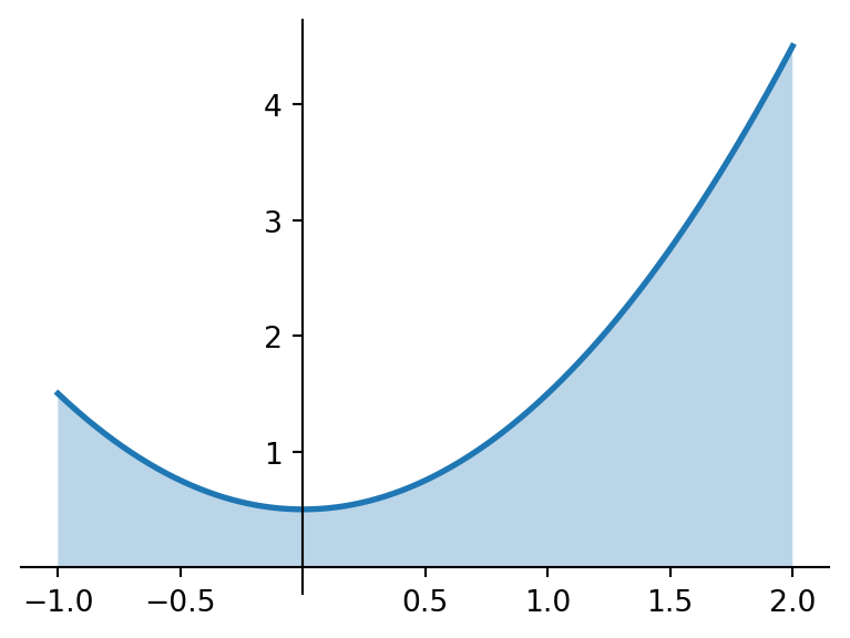
When you read the word ‘integration’ most or even all of you will immediately think back to the integral you have learned about in your earlier studies: the Riemann integral to call it by its full name. Given some (suitable) non-negative¹ function $f:[a,b] \to [0,\infty)$ we denote it by \[\int_a^b f(x) \d x \tag{3.1}\] and it has some value in $[0,\infty]:=[0,\infty) \cup \{\infty\}$ that we can naturally interpret as “the area under the graph of $f$” (i.e. the area of the region enclosed by the lines $x=a$ and $x=b$, the horizontal axis, and the graph of $f$). We typically compute its value as $F(b)-F(a)$, where $F$ is any antiderivative of $f$. Obligatory figure for illustration:

¹ Of course, as we know well we don’t need to limit ourselves to non-negative functions only but it is a natural place to start this discussion

Figure 3.1: The graph (dark blue) of $f(x)=x^2+1/2$ on the interval $[-1,2]$; and the area of the light blue region equals $\int_{-1}^2 x^2+1/2 \d x=4.5$

Obviously Riemann integrals are very important and are natural to use in many applications. However, and here is the mathematician’s desire for generalisation again, it turns out that you can extend the thinking behind this concept in several ways to construct a large zoo of many kinds of more exotic types of integrals:

you can integrate functions with codomain $\R$, like the Riemann integral does, but in a different way and/or with different domains than $\R$
you can integrate more complicated objects as well, not just functions!

In this course we will not touch on point 2. (within the Probability Theory context, you may very well encounter for instance stochastic integration in a different course) but we will spend this chapter exploring point 1.

Briefly about the global idea behind point 1 (don’t worry about this brief discussion and Proposition 3.1 for exam purposes). Let’s fix some $a$ and $b$. What does the Riemann integral actually do? Well, you choose a (suitable) function $f$ and compute its integral i.e. obtain a number. So essentially it is nothing but a mapping, say $I$, that has as domain some large set of suitable functions and maps these to a real number (typically $\pm \infty$ are allowed as well, see further below). For example, if we let $I_R$ be the Riemann integral for functions $[0,1] \to \R$, then for $f(x)=x$ we get $I_R(f)=1/2$. There are some fundamental properties that an expert would tell you every sensible concept of integral should have:

Proposition 3.1 In general an integral is a mapping $I$ with as domain some suitable family of real valued functions, say $\mathbf{D}$, that maps to $\R$ with the following defining properties:

linearity: $I(\alpha f+ \beta g)=\alpha I(f)+\beta I(g)$ for $\alpha,\beta \in \R$,
non-negativity: if $f$ is non-negative then $I(f) \geq 0$,
continuity: if $f_1 \geq f_2 \geq \ldots$ is a non-increasing sequence of non-negative functions so that $f_n \downarrow 0$ as $n \to \infty$ (pointwise) then also $I(f_n) \downarrow 0$ as $n \to \infty$.

It is not hard to see that these defining properties imply the following two properties (cf. Exercise 3.1):

if $f \leq g$ then $I(f) \leq I(g)$,
if $f_1 \leq f_2 \leq \ldots$ is a non-decreasing sequence of functions so that $f_n \uparrow f$ as $n \to \infty$ (pointwise), then also $I(f_n) \uparrow I(f)$ as $n \to \infty$.

Some notes:

In all the above, we conveniently assume that whatever expression we plug into $I$ is actually an element of $\mathbf{D}$. It can be made more precise what properties $\mathbf{D}$ should exactly have to be useful in this context, see e.g. Chapter VII in Stroock (1994).
Property 2 is in particular inspirational, it gives rise to the following strategy for constructing a new integral: identify within your $\mathbf{D}$ an easy to understand family of non-negative functions for which you can easily write down what value your integral should have, and that allows you to pointwise approximate any other non-negative function in $\mathbf{D}$, so that via property 2 the integral value for any non-negative function follows. The extension to any function is then a matter of considering its so-called positive and negative parts separately (using linearity i.e. property i). Indeed this is the strategy we’ll also be following in this chapter!
Generally we want to slightly extend this concept by allowing for integral values of $\pm \infty$ as well, in particular in property 2 it is natural to set $I(f)=\infty$ for cases where $\lim_{n \to \infty} I(f_n)=\infty$.

But, and this is what point 1 above is referring to, the Riemann integral is far from the only choice you could make: there are many other choices for mappings in the vein of Proposition 3.1 — there is not just the Riemann integral, but many ‘other integrals’ (working on functions) exist as well!

The setting in this chapter is a probability space $(\Omega,\mathcal{F},\P)$ (cf. Definition 2.3) on which we consider random variables i.e. measurable (cf. Definition 2.1) functions $X: \Omega \to \R$ for which we would like to define an integral. Until we get to Section 3.4, we don’t care much about the Probability Theory interpretation involving random experiments etc. — indeed $(\Omega,\mathcal{F},\P)$ is “just” a measure space and $X$ is “just” a measurable function for which we would like to define a new type of integral. I am stressing this because this task of defining a new integral is all measure theory and applies identically to any measure space $(E,\mathcal{F},\mu)$ — just replace in our discussion of the new integral everywhere “$\Omega$” by “$E$” and “$X$” by “$f$” (as the more general symbol for a function). Recall that the only non-cosmetic difference is that a probability space has the special property that the whole universe has measure $1$ while for a general measure space it can be anything positive (incl. infinity).

But why do we spend time on integration in the context of this course? Well the reason is that this new type of integral will allow us to establish a new, more general understanding of how we should define and compute the expectation of any random variable $X$, consistent with the formulae we’re already familiar with for discrete and continuous random variables (Section 2.5.1), but also covering any ‘other’ ones! An interesting thought maybe: as we also saw in Section 2.5.1, in the expressions for expectation we know already we use a summation in the discrete case and an integral in the continous case. This paragraph suggests, and we will indeed see, that no matter how different they may seem, they are in fact both special cases of one single new type of integral! :).

Exercises

You can now do Exercise 3.1.

3.2 A little bit of preparation

Before we carry on with the main story line, first two little intermezzos to discuss some stuff that will be very useful later on. In this section we’ll just use the symbol “$f$” for a function rather than “$X$”, just because it’s less awkward (I think). But that’s cosmetics only obviously.

3.2.1 The positive and negative part of a function

In the context of constructing/working with integrals, it is convenient to be able to focus on functions with only one sign, say only non-negative. To faciliate this, any function $f:\Omega \to \R$ naturally splits up in what we call its positive part and its negative part, both non-negative functions. To get its positive part, you take $f$ and whenever it has a negative value you adjust that to $0$. This creates a new function which we denote by $f^+$. To get its negative part, denoted by $f^-$, you take $f$ and

whenever it has a positive value you adjust that to $0$,
whenever it has a negative value you multiple it by $-1$

(so, the negative part is actually a non-negative function due to that multiplication by $-1$!).

In mathematical terms, the functions $f^+, f^-:\Omega \to [0,\infty)$ are hence defined as follows: for any $x \in \Omega$ \[f^+(x) := \begin{cases} f(x) & \text{if $f(x)>0$} \\ 0 & \text{if $f(x) \leq 0$} \end{cases} = \max\{f(x),0\} \tag{3.2}\] and \[f^-(x) := \begin{cases} -f(x) & \text{if $f(x)<0$} \\ 0 & \text{if $f(x) \geq 0$} \end{cases} = \max\{-f(x),0\}. \tag{3.3}\]

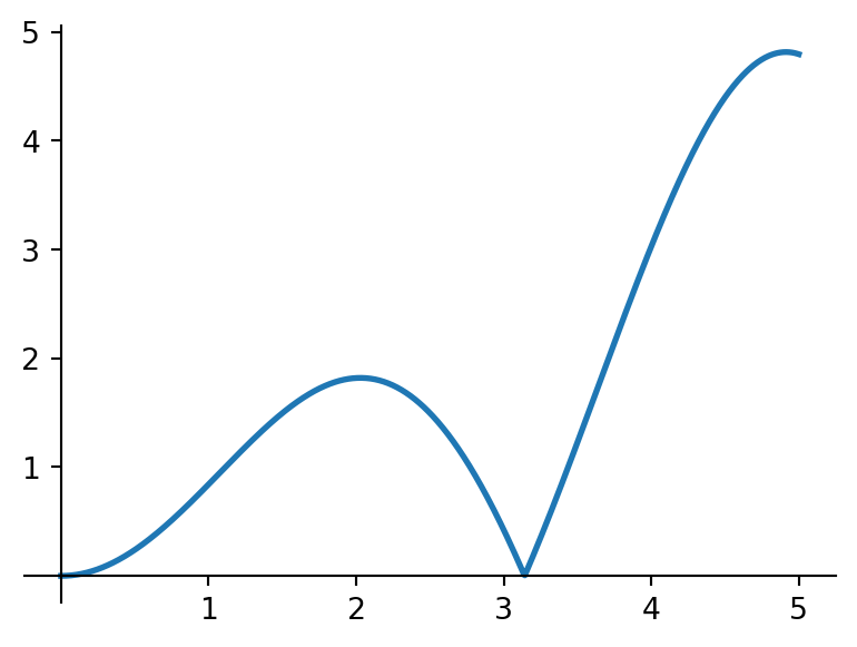
Visually it is immediately clear what is going on — take for example the function $f(x)=x \sin(x)$ on $\Omega=[0,5]$, which looks as follows:

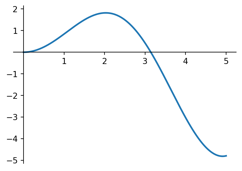
Figure 3.2: The graph of $f(x)=x \sin(x)$ on $\Omega=[0,5]$

then this is what the two parts look like (note also that the negative part of $f$ is the same as the positive part of $-f$):

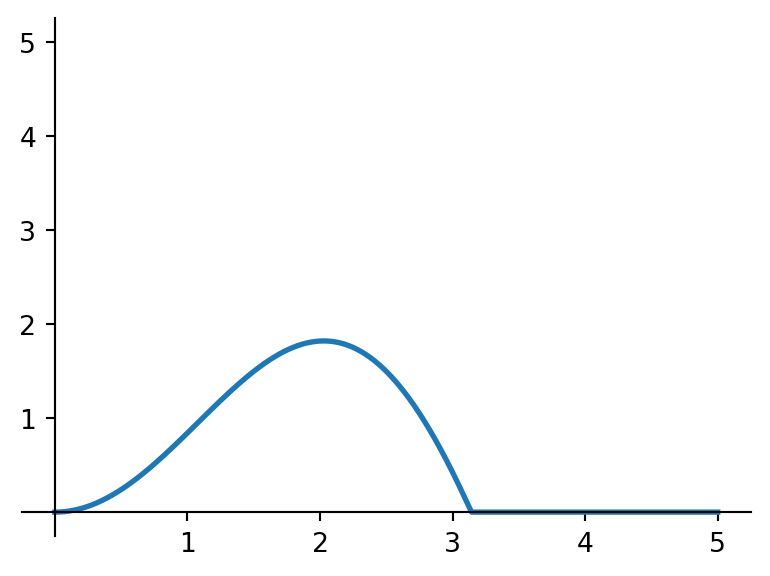
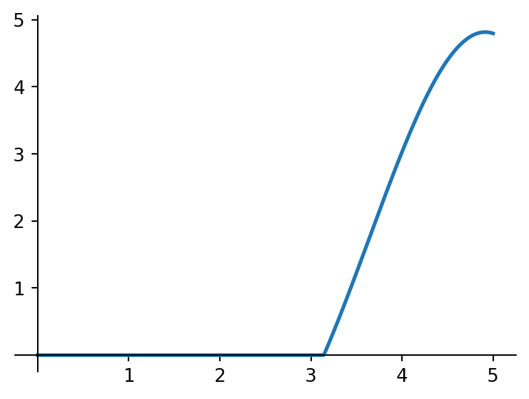
You can easily gaze that we have the following handy relationships:

Proposition 3.2 Given a function $f:\Omega \to \R$ with its positive and negative parts $f^+, f^-$ as defined in Equation 3.2 and Equation 3.3, we have for any $x \in \Omega$:

$f(x)=f^+(x)-f^-(x)$,
$|f(x)|=f^+(x)+f^-(x)$.

Indeed, going back to our example to visually illustrate point ii above, if we add together the two graphs from Figure 3.3 then we get Figure 3.4:

Figure 3.4: The graph of $x \mapsto |f(x)|=|x \sin(x)|$ as well as $x \mapsto f^+(x)+f^-(x)$ on $\Omega=[0,5]$

Here is how these guys are useful for us. For a function $f: \Omega \to \R$, using that $f=f^+-f^-$ (cf. Proposition 3.2 i) and the fact that we want our integral to be linear (cf. Proposition 3.1 i), the integral for $f$ is naturally given by the integral for $f^+$ minus the integral for $f^-$. So when defining a new integral, it is enough to focus on non-negative functions only and then apply this logic to extend it to any function. And working with non-negative functions only, we don’t have to worry about how to balance out positive and negative values of a function in our integral, that’s all automatically taken care of (where possible) by this extension idea!

And in fact, you already know/use this principle for good old Riemann integrals as well (though you would be forgiven for not having that very sharp anymore)! The below example briefly discusses this.

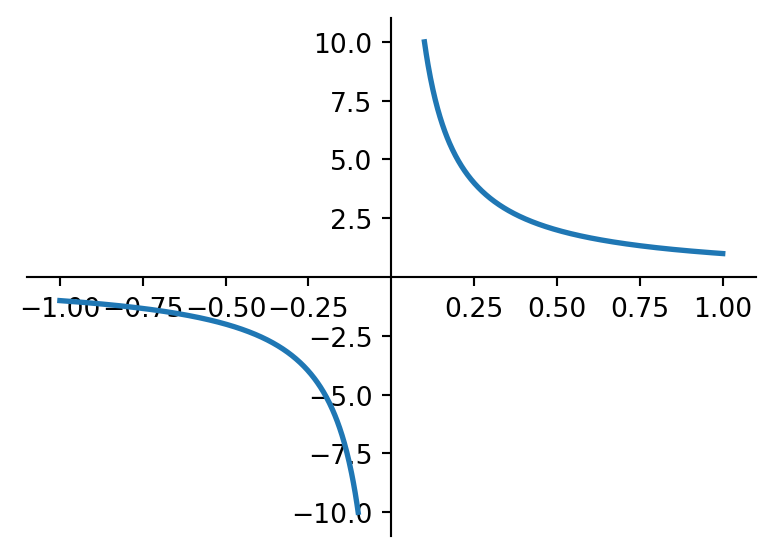
Example 3.1 Take the function $f(x)=1/x$ for $x \not=0$ and say $f(0)=0$ (the value in $0$ is not relevant for the below, we just choose something). Cf. Figure 3.5. Let’s consider the good old Riemann integral for this function on some different intervals.

Firstly, as is hopefully readily clear, its positive and negative parts look as follows: \[f^+(x) = \begin{cases} 1/x & \text{if $x>0$} \\ 0 & \text{if $x \leq 0$} \end{cases} \quad \text{and} \quad f^-(x) = \begin{cases} -1/x & \text{if $x<0$} \\ 0 & \text{if $x \geq 0$} \end{cases}\]

In principle (as mentioned above, you may well not have this very sharp anymore), for Riemann integrals we also use the principle that for any $f$ we define \[\int_a^b f(x) \d x := \int_a^b f^+(x) \d x - \int_a^b f^-(x) \d x \tag{3.4}\] so that we only need to understand how to integrate non-negative functions as that is enough to work out the right hand side. Let’s see what this looks like for some different choices of the interval $[a,b]$.

First consider $[a,b]=[0,1]$. There we get, as you can readily check \[\int_0^1 f^+(x) \d x = \int_0^1 1/x \d x=\infty \quad \text{and} \quad \int_0^1 f^-(x) \d x = \int_0^1 0 \d x=0\] and hence Equation 3.4 gives us \[\int_0^1 f(x) \d x=\infty-0=\infty.\]

Similarly if we consider $[a,b]=[-1,0]$, then we get \[\int_{-1}^0 f^+(x) \d x = \int_{-1}^0 0 \d x=0 \quad \text{and} \quad \int_{-1}^0 f^-(x) \d x = \int_{-1}^0 -1/x \d x=\infty\] and hence in this case Equation 3.4 gives us \[\int_{-1}^0 f(x) \d x=0-\infty=-\infty.\]

Now let’s make it a bit more interesting by considering the interval $[a,b]=[-1,1]$. Then \[\int_{-1}^1 f^+(x) \d x = \int_{0}^1 1/x \d x = \infty \quad \text{and} \quad \int_{-1}^1 f^-(x) \d x = \int_{-1}^0 -1/x \d x=\infty.\] If we now again try to go back to Equation 3.4 to get the integral for $f$ we end up with $\infty-\infty$ which, as you’ll remember, cannot be given a (consistent) meaning i.e. is undefined. So we are forced to conclude that \[\int_{-1}^1 f(x) \d x \text{ does not exist/is not well defined!}\]

Arguing via the “integral is area of the region under the graph of $f$” principle: on the interval $[0,1]$ we have an area of $\infty$, on $[-1,0]$ we have an area of $-\infty$ (that’s how it works for negative functions!), and hence the area on $[-1,1]$ is undefined as it forces us to add both these areas i.e. to evaluate $\infty-\infty$.

The key take away of this example is this: as long as at least one of $f^+$ and $f^-$ has a finite integral we’re fine and the integral of $f$ is well defined via Equation 3.4 (though it may well be $-\infty$ or $\infty$ of course). If both have an infinite integral though then we’re out of luck and need to consider the integral of $f$ as undefined/non-existent. We’ll use this line of argument in exactly the same way for our new integral!

3.2.2 The Riemann integral as the “average value” of a function

When you construct a new integral, as we do in this chapter, then you do that with a certain philosophy in mind: your integral has a certain interpretation/meaning — in fact the whole purpose of constructing an integral is to put that interpretation/meaning into maths. In our case, we will later see that we give our new integral the interpretation/meaning that it equals the “average value” of the real valued function that we’re integrating.

I would guess that for most of you, the natural interpretation of the Riemann integral of a non-negative function $f$ is “the area under the graph of $f$” as also discussed at the start of this chapter. In this section I would like to try and convince you (if necessary) that you can equally well interpret a Riemann integral as giving the “average value” of $f$ (in the process we’ll also need to clarify what that exactly means!). The intuition and understanding about the average value of a function that we build up as we do this will be very beneficial in the rest of this chapter as well!

Let’s first briefly recall what we know about the concept of average values more generally. The most basic case is that of a set of good old numbers, say $a_1, \ldots, a_n$. In that case we all know well that its average value is given by \[\frac{1}{n} \sum_{k=1}^n a_k. \tag{3.5}\] The process of computing the average value essentially maps the set of numbers to a single number, and not just any old number: it is the typical answer to the question “If you have to pick a single number that best represents the values in your sequence, what number would that be?”. In the context of data analysis, for any set of data its average is typically the most prominent metric (or “statistic” in that context).

We’re also all familiar with the concept of a weighted average i.e. we have a set of numbers $a_1, \ldots, a_n$ as above but now we also have non-negative weights $w_1,\ldots,w_n$. Without loss of generality we may assume that they sum up to $1$². Then the natural extension of the average value in Equation 3.5 is the weighted average value i.e. \[\sum_{k=1}^n w_k a_k. \tag{3.6}\] The idea is: the larger $w_k \in [0,1]$, the “more important” we consider the number $a_k$ in the sequence and the more influence that number will have on the average. Indeed, in the extreme case that $w_k=1$ for some $k=1,\ldots,n$ all the other weights must be $0$ (as they add up to $1$) and hence the weighted average Equation 3.6 boils down to $a_k$.

² If they don’t, then simply “normalise” each weight by dividing it by the sum of weights

Note that Equation 3.6 is a generalisation of Equation 3.5 in the sense that if all weights are equal i.e. if $w_k=1/n$ for $k=1,\ldots,n$, then Equation 3.6 simplifies to Equation 3.5.

Coming from this angle, take a non-negative function $f:[a,b] \to [0,\infty)$ (as discussed in Section 3.2.1 we can focus on non-negative functions). Where above we wrote “average value” of $f$, we mean more specifically the “average value” of the set of values that $f$ takes in its codomain $[0,\infty)$ i.e. the “average value” of the range of $f$ (recall from Section 2.2) i.e. the “average value” that $f$ takes, with awareness for how we should weigh the values in the range. Visually speaking, this is the “average value” of all values that the graph of $f$ visits on the vertical axis if you will. We’re stubbornly writing quotes around “average value” because of the following: as long as we have a finite (or countably infinite) set of numbers (in the range of $f$), then the (weighted) average is perfectly well defined by Equation 3.5 and Equation 3.6. However it’s less obvious what “average value” should mean if the set of numbers (range of $f$) is uncountable, hence the reservation for now.

Ok. As mentioned above, the goal is to convince you that, no matter whether the range of $f$ is countable or uncountable, we can naturally understand/interpret/define this “average value” in terms of the Riemann integral, specifically:

Proposition 3.3 For any function $f:[a,b] \to \R$ (whose Riemann integral exists) we can naturally understand/define \[\text{the average value that $f$ takes} = \frac{1}{b-a} \int_a^b f(x) \d x \tag{3.7}\] (provided that this Riemann integral exists).

Rather than throwing (only) a formal argument at this, let me try to convince you more at an intuitive level. First consider a constant function, say $f(x)=c$. Then the range of $f$ is of course just the set containing that single element: $\{c\}$. What is the average value if we have only a single number? Well just the number itself i.e. $c$ no? This is of course just Equation 3.5 with $n=1$. We can readily check that in this case $\int_a^b f(x) \d x=c (b-a)$ and hence Equation 3.7 indeed holds.

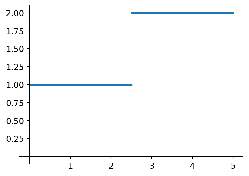
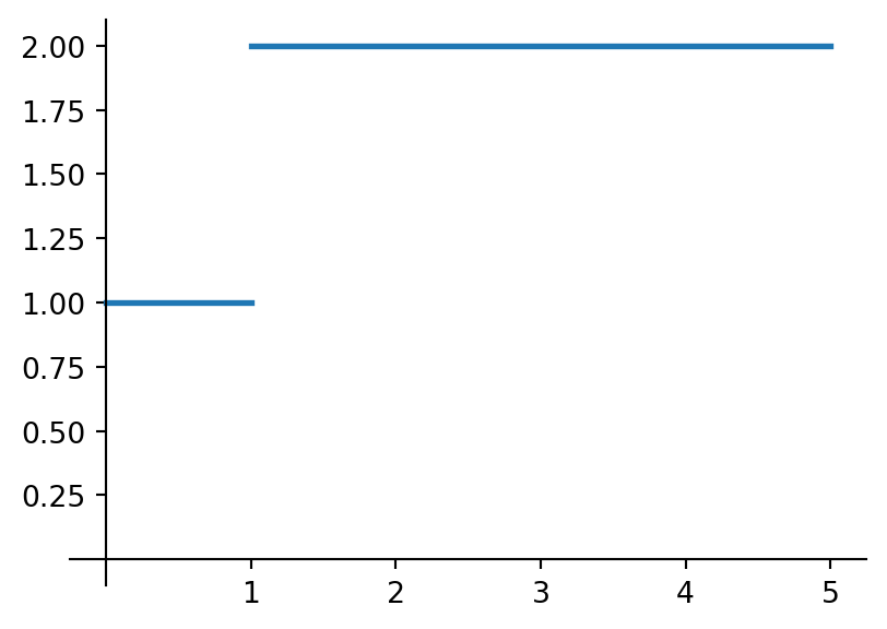
Next let’s consider a function taking only two values, say $1$ and $2$ so with range $\{1,2\}$. Two such functions, $f_1$ and $f_2$, are shown in Figure 3.6. As first stab, purely based on the range, could we say that the average value taken is $1.5$ for both functions? For $f_1$, yeah that makes sense. However for $f_2$ that feels a bit wrong I hope you’ll agree: you’d feel that the average value should be larger because it spends “longer” at the value $2$ than at the value $1$ (while for the first one it’s equally “long” for both values) no. To express this more precisely, look at the horizontal axis: $f_1$ maps equally long³ intervals to both values: $[0,2.5)$ to $1$ and $[2.5,5]$ to $2$, but for $f_2$ the lengths are different: $[0,1)$ to $1$ and $[1,5]$ to $2$. The natural way to account for this difference is to use the lengths of these intervals as weights to create a weighted average.

³ We don’t care about a single point difference. What is that, does this “length” business remind you of the Lebesgue measure from Section 1.6.1? Well I can promise you already that that’s not a coincidence!

⁴ If integrating such a discontinuous function feels too unusual to you, just split the integral up over the different intervals where these functions are constant

This would look as follows: the domain of both functions is $[0,5]$ i.e. has total length $5$, and we create weights by looking at the lengths of the above intervals relative to this total length. That is to say, for $f_1$ the average value becomes \[\frac{2.5}{5} \cdot 1 + \frac{2.5}{5} \cdot 2=1.5\] (so still $1.5$ here, as expected) while for $f_2$ the average value becomes \[\frac{1}{5} \cdot 1 + \frac{4}{5} \cdot 2=1.8\] (a larger value than $1.5$, as we wanted). I hope that you agree that intuively this way of computing the average value makes a lot of sense. Furthermore, as you can easily check by working out⁴ $\int_0^5 f_1(x) \d x$ and $\int_0^5 f_2(x) \d x$, for both $f_1$ and $f_2$ the right hand side of Equation 3.7 also equals $1.5$ and $1.8$ resp., so Equation 3.7 holds for $f_1$ and $f_2$ as well, so we’re still going strong with making our argument that Proposition 3.3 indeed makes sense!

(a) The function $f_1:[0,5] \to [0,\infty)$ given by $f_1(x)=1$ if $x < 2.5$ and $f_1(x)=2$ if $x \geq 2.5$

This idea immediately generalises to a very prominent class of functions that we like to call step functions. Suppose that $f:[a,b] \to [0,\infty)$ is created as follows: cut up (=partition) the domain $[a,b]$ into intervals $I_1, \ldots, I_n$⁵, and let $f$ be constant with value $y_i$ on each interval $I_i$. Note that $f_1$ and $f_2$ above were specific examples of such step functions (with $n=2$), and the constant function we first considered was also one (trivially, with $n=1$). Now the range of $f$ is $\{y_1,\ldots,y_n\}$, and applying the above logic that the average value of $f$ should be the average of these $y_i$’s but weighted for the lengths of the corresponding intervals, each $y_i$ should get as weight the length of its corresponding interval $I_i$ as a fraction of the length of the whole domain i.e. $b-a$ (note that this makes the weights nicely add up to $1$). That is to say, the average value of $f$ is naturally given by \[\frac{\text{length of } I_1}{b-a} y_1 + \frac{\text{length of } I_2}{b-a} y_2 + \ldots + \frac{\text{length of } I_n}{b-a} y_n. \tag{3.8}\] And yes, as you can again easily check, by working out $\int_a^b f(x) \d x$, with this choice Equation 3.7 still holds!

⁵ Recall from into Section 1.2.3, e.g. just take some points $a=x_0<x_1<x_2<\ldots<x_n=b$ and set $I_i=[x_{i-1},x_i)$ for $i=1,\ldots,n-1$ and $I_n=[x_{n-1},x_n]$

Even though this class of step functions is prominent (as we will see later as well) and it is very good to have them on board, there are many other functions as well of course. In particular such a step function has a finite range while in general a function can of course very well have an infinite and indeed even uncountable range (in which case the whole concept of its average value is less obvious, as already mentioned above).

To convince ourselves that Proposition 3.3 makes sense for general functions as well, here’s two ways forward. A more rigorous approach is to remind yourself about how Riemann integrals are defined/constructed, namely as a limit of “lower sums”/“upper sums” (see e.g. Wiki), and these are nothing but particular examples of step functions as defined above. Then you take the limit, and essentially define the average value of a general function as the limit of the average values of approximating step functions⁶.

⁶ This seems too indirect/too much cheating to be convincing to you? Ok. Are you convinced about the Riemann integral=area of the region under the graph principle? But that suffers from the same problem: if you have some wiggly function, exactly how is “area of the region under the graph” defined/expressed? I mean, I know expressions for the areas of triangles, rectangles and you name it, but not for arbitrary shapes. So yes, in fact the only way to define/express the “area of the region under the graph” in general is via its association with the Riemann integral/as a limit of the areas under the graphs of approximating step functions — exactly the same philosophy as we follow here for “average value”!

Alternatively, here is an attempt at a cute analogy. If you drive on your bike through Manchester, how do you compute your average speed? Well by dividing the distance travelled by how long the drive took you. In other words, that average speed is exactly the speed needed to make the same trip in the same time if you were to travel at constant speed. Hold that thought.

Now imagine that in the garden of your student flat, for the summer you have set up for a nice cuboid shaped swimming pool. You’re standing in front of your pool. Imagine a horizontal axis running along the bottom of the front of the pool, with the pool starting at $x=a$ and ending at $x=b$.

Sadly the day is cold and very windy (not at all common here in Manchester of course), so there are waves in your swimming pool: the water is higher in some places than in others. What is the average height of the water? That is exactly the height the water would have if it were perfectly smooth with no waves at all. Why? Because the volume of the water doesn’t change, and the average height is exactly the water height you need to fill the pool with the same amount of water if the height is constant everywhere (analogue to the average speed on your bike).

Now think about your function $f:[a,b] \to \R$. Imagine that the graph of $f$ describes exactly what the waves look like: for any $x \in [a,b]$ the height of the water at position $x$ is given by $f(x)$. The volume of the water with waves is then the area under the graph of $f$ multiplied by the length of the pool, say $l$, i.e. \[l \int_a^b f(x) \d x.\] When the water is in rest, by the above argument the constant height of the water, say $h$, is the average height of the water with waves and hence also the average value of your function $f$. The volume of the water is now given by the pool width $b-a$ times constant water height $h$ times the length of the pool $l$: $(b-a) h l$.

Using that the volume of the water in rest is the same as the volume of the water with waves, we can work out what $h$ is: \[l \int_a^b f(x) \d x=(b-a) h l \quad \implies \quad h=\frac{1}{b-a} \int_a^b f(x) \d x.\] Oi, that’s exactly Proposition 3.3!

Exercises

You can now do Exercise 3.2.

3.3 Lebesgue integrals

Ok, back to the main storyline now. Here is the situation: we have a probability space $(\Omega,\mathcal{F},\P)$ on which measurable functions $X: \Omega \to \R$ i.e. random variables live. We want to define a new type of integral that acts on such functions $X$ and maps them to a value in $\R$ (allowing for $\pm \infty$ as well) in the sense of Proposition 3.1. Our purpose is to create this new integral with a particular interpretation: we want it to represent the average value of $X$ (as shorthand for the average of the values in the range of $X$, properly weighted (somehow)).

In Section 3.2.2 we already discussed this idea of average value for functions that have (an interval in) $\R$ as their domain and saw how we could use the Riemann integral for it. Now we want to do this for functions on a more general universe $\Omega$ (as part of a measure space/probability space structure). Note that the focus is very much on reasoning from the perspective of the range of the function which is still some set in $\R$, as it also was in Section 3.2.2. The difference with Section 3.2.2 is “only” that the domain $\Omega$ is now a general set, no longer necessarily (an interval on) the real line. However, if you think back to Section 3.2.2 then we used the domain of the function only to determine appropriate weights for the values in its range, and it turns out that this functionality can quite easily be replicated by an $\Omega$ that is part of a probability space!

We’ll call our new integral the Lebesgue integral and let us for the time being denote it by $I_L$ (we’ll give it fancier notation later on). We’ll break our construction task up in a number of steps, as follows:

Define $I_L$ on a class of non-negative step functions (that are easy to understand and easy to give a value).
Use approximation by step functions to define $I_L$ for any non-negative function (essentially relying on property 2 in Proposition 3.1).
For any function, let $I_L$ act on its positive and negative part to define, whenever possible, $I_L$ for the function itself (following the same ideas as in Section 3.2.1).
Conclusion of the first three steps, more fancy notation and some properties of Lebesgue integrals.
Quick look at Lebesgue integrals vs Riemann integrals.

Grab a few cans of Diet Coke, here we go!

3.3.1 Step 1: non-negative step functions

Recall that in Section 3.2.2 we already looked at step functions on the domain $[a,b]$: partition the domain into finitely many subintervals and take a function that is constant on each subinterval, which creates a function with a finite range i.e. which has only finitely many possible values.

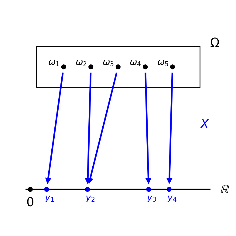
We want to do the analogue thing in our more general context of functions that have the universe $\Omega$ as domain, working from the codomain/range of the function backwards. Let $X: \Omega \to [0,\infty)$ be any measurable non-negative function on $(\Omega,\mathcal{F},\P)$ with finite range, say $\{y_1,\ldots,y_n\} \subseteq [0,\infty)$. We call this a step function.

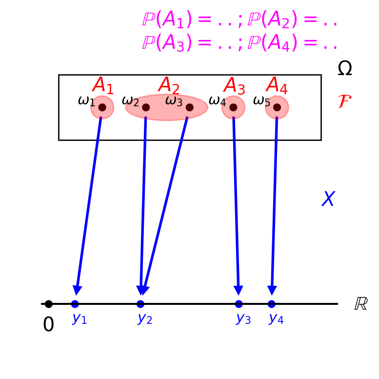
Note that the inverse images $X^{-1}(\{y_1\}), \ldots, X^{-1}(\{y_n\}) \in \mathcal{F}$ form a partition of $\Omega$ (every $\omega \in \Omega$ gets mapped to one of the $y_i$’s and is hence an element of exactly one of these inverse images, mild variation of Lemma 2.1 ii). Recall also Example 2.1. If for convenience we write $A_i=X^{-1}(\{y_i\})$, then we can express $X$ as \[X(\omega)=\begin{cases} y_1 & \text{if $\omega \in A_1$} \\ y_2 & \text{if $\omega \in A_2$} \\ \vdots & \\ y_n & \text{if $\omega \in A_n$} \end{cases} =\sum_{i=1}^n y_i \mathbf{1}_{A_i}(\omega) \tag{3.9}\] where $\mathbf{1}_{A_i}$ denotes an indicator function as already introduced in Exercise 2.3. If the second equality confuses you, note that it is trivially true (it’s just an alternative, more compact notation really): if you fix any $\omega \in \Omega$, then only exactly one of these indicator functions has the value $1$ (indeed, the one for the event $A_i$ that $\omega$ is an element of) and all the other indicator functions have the value $0$. So only one term in that summation is not $0$, and it has the value $y_i$.

Of course, you could conversely also start with cutting up $\Omega$ into a partition $A_1, \ldots, A_n \in \mathcal{F}$, choose non-negative values $y_1, \ldots, y_n$ and create a (measurable, non-negative) step function $X$ by defining it like Equation 3.9 (we encountered this guy before in Exercise 2.3).

On to the main question: for such a step function $X$ with range $\{y_1,\ldots,y_n\} \subseteq [0,\infty)$, what should $I_L(X)$ be i.e. the value that our new integral gives $X$ i.e. the average value of $X$? In Section 3.2.2 we said that the average value of a step function should be the average value of its range, but with weights accounting for the lengths of the subintervals corresponding to each $y_i$ (cf. Equation 3.8). Note that in this case, it’s these inverse images $X^{-1}(\{y_1\}), \ldots, X^{-1}(\{y_n\})$ that play the role of these subintervals (they make up the sets in the domain $\Omega$ on each of which $X$ is constant). So we want to weigh each $y_i$ in the range with the “size” of the corresponding inverse image $X^{-1}(\{y_i\})$ relative to the “size” of whole domain $\Omega$.

Oi, we remember that “size” business from somewhere! Well indeed, as discussed in Section 1.5, that’s exactly why we have a (probability) measure $\P$ as part of our measure/probability space, to give meaning to the “size” of (suitable) subsets of $\Omega$! So, using $\P$, the last sentence of the previous paragraph means that we want to give each $y_i$ in the range the weight $\P(X^{-1}(\{y_i\}))/\P(\Omega)$. You can easily double check, using that these inverse images form a partition of $\Omega$ and countable additivity (cf. Definition 1.3), that these weights indeed sum up to $1$.

So, the range contains the values $y_1,\ldots,y_n$, with corresponding weights \[\frac{\P(X^{-1}(\{y_1\}))}{\P(\Omega)}, \ldots, \frac{\P(X^{-1}(\{y_n\}))}{\P(\Omega)}\] and we want our new integral $I_L(X)$ to be the corresponding weighted average (as in Equation 3.6), so we naturally arrive at the following definition: \[I_L(X) := \frac{\P(X^{-1}(\{y_1\}))}{\P(\Omega)} y_1 + \frac{\P(X^{-1}(\{y_2\}))}{\P(\Omega)} y_2 + \ldots + \frac{\P(X^{-1}(\{y_n\}))}{\P(\Omega)} y_n.\]

That’s it for non-negative step functions! All that remains is to clean this up a tiny bit: note that since we’re on a probability space we conveniently have $\P(\Omega)=1$ and using our usual ‘lazy’ shorthand to write $\P(X=y_i)$ for $\P(X^{-1}(\{y_i\}))$. So:

Definition 3.1 If $X: \Omega \to [0,\infty)$ is a measurable function on $(\Omega,\mathcal{F},\P)$ with finite range $\{y_1,\ldots,y_n\} \subseteq [0,\infty)$, then we define its Lebesgue integral $I_L(X)$ as \[I_L(X):=\sum_{i=1}^n y_i \P(X=y_i) \in [0,\infty).\]

As a useful special case, note that for any $A \in \mathcal{F}$ we have that \[I_L(\mathbf{1}_A)=\P(A).\]

We can naturally understand/interpret $I_L(X)$ as the average value that $X$ takes on the real line.

If you don’t immediately see the second expression, just note that $\mathbf{1}_A$ has range $\{0,1\}$ and $\mathbf{1}_A(\omega)=1$ if and only if $\omega \in A$ i.e. in terms of inverse images: $\{\mathbf{1}_A=1\}=A$ and $\{\mathbf{1}_A=0\}=A^c$, so \[I_L(\mathbf{1}_A)=0 \cdot \P(\mathbf{1}_A=0)+1 \cdot \P(\mathbf{1}_A=1)=0 \cdot \P(A^c)+1 \cdot \P(A)=\P(A).\]

Note: there is a small question of consistency due to non-unique representation of such a step function here, but that’s easily resolved, see e.g. Lemma 3.2.3 in Stroock (1994).

If you’d like a visual, see Figure 3.7 below.

(a) The setup as in Figure 2.2 where we now label the values on the real line $y_1,\ldots,y_4$ — as these are all non-negative this $X$ is a non-negative step function

Exercises

You can now do Exercise 3.3.

3.3.2 Step 2: any non-negative function

Next stop: any non-negative measurable function $X: \Omega \to [0,\infty)$. We’re looking to utilise the desired property 2 in Proposition 3.1 of our new integral: we are looking for a sequence of non-negative step functions, say $X^{(n)}$ for $n=1,2,\ldots$ so that for all $\omega \in \Omega$ we have $X^{(1)}(\omega) \leq X^{(2)}(\omega) \leq \ldots$ and $X^{(n)}(\omega) \uparrow X(\omega)$ as $n \to \infty$. Then we can simply define the integral of $X$ i.e. $I_L(X)$ as the limit of $I_L(X^{(n)})$ (which we know how to compute from Definition 3.1) as $n \to \infty$.

It is intuitively obvious (just a bit annoying to write down a precise argument for) from Definition 3.1 that because the $X^{(n)}$’s are pointwise non-decreasing, the sequence of integral values $I_L(X^{(1)}), I_L(X^{(2)}), \ldots$ forms a non-decreasing sequence of non-negative numbers which is hence guaranteed to have a non-negative limit (it may be $\infty$ though).

Ok… Bit of Q&A:

Is there no easier way? Well not with the same reach at least — this is a very common step in such constructions! And it allows us to handle any non-negative function, including those with uncountable ranges etc., no small feat!
Why is this the right way of doing it, why not approximate $X$ in some different way for instance? Well, as already mentioned, given such $X^{(n)}$’s we know that $I_L(X)$ has to be be the limit of the $I_L(X^{(n)})$’s — if it were anything else then we would be constructing an integral that violates property 2 in Proposition 3.1 i.e. something that is not a “sensible” integral.
Can we still interpret $I_L(X)$ as the average value that $X$ takes on the real line? Yes, if you agree that it makes sense for the concept of average value to be “continuous” in the sense that if two functions get arbitrarily close together, then so do their average values. That same principle is used to establish the interpretation that the Riemann integral gives the area of the region under the graph of any non-negative function though, so if you’re happy to accept that then this is no different!

Showing that we can create a sequence of step functions with the properties we’d like is not very difficult, just a bit tedious.

Remark 3.1. Here is a way to create such a construction (don’t worry about it for exam purposes). Fix some $n=1,2,\ldots$. Partition the codomain $[0,\infty)$ of $X$ into $4^n+1$ parts/intervals, as follows: $B^{(n)}_k=[k/2^n,(k+1)/2^n)$ for $k=0,\ldots,4^n-1$ and $B^{(n)}_{4^n}=[2^n,\infty)$. Their inverse images $A^{(n)}_k:=X^{-1}(B^{(n)}_k)$ then form a partition of $\Omega$ (cf. Lemma 2.1). Now let $X^{(n)}$ be the step function that is constant on each $A^{(n)}_k$, taking the value $k/2^n$ there: \[X^{(n)}(\omega) = \sum_{k=0}^{4^n} \frac{k}{2^n} \mathbf{1}_{A^{(n)}_k}(\omega)\] (recall this expression using indicator functions from Equation 3.9).

Let’s briefly discuss that this construction works in the way intended. First note on each $A^{(n)}_k$, $X^{(n)}$ takes the value $k/2^n$ while $X$ has there as smallest value $k/2^n$ (by def of $B^{(n)}_k$), so indeed $X^{(n)} \leq X$ (pointwise and for all $n$). Fix any $\omega \in \Omega$ and set $y=X(\omega) \in [0,\infty)$. Then for all $n$ large enough (so that $2^n>y$), $y \in B^{(n)}_k$ for the $k$ that satisfies $k/2^n \leq y < (k+1)/2^n$. That means that $X(\omega)-X^{(n)}(\omega)=y-k/2^n<1/2^n$ which vanishes as $n \to \infty$, so indeed $X^{(n)} \uparrow X$ pointwise as $n \to \infty$. Finally (and here is where the reason for choosing these maybe awkward looking powers of $2$ becomes clear), if we make the step from $X^{(n)}$ to $X^{(n+1)}$, then each interval $[k/2^n,(k+1)/2^n)$ in the partition at step $n$ splits into two new intervals in the partition at step $n+1$, namely $[l/2^{n+1},(l+1)/2^{n+1})$ and $[(l+1)/2^{n+1},(l+2)/2^{n+1})$, where $l=2k$. This means that on the set in $\Omega$ where $X^{(n)}$ was constantly equal $k/2^n$, $X^{(n+1)}$ has two possible values: $2k/2^{n+1}$ and $(2k+1)/2^{n+1}$ i.e. $k/2^n$ and a value larger than $k/2^n$ but smaller than $(k+1)/2^n$. This shows that this particular way of “refining” the partition as $n$ grows ensures that $X^{(1)} \leq X^{(2)} \leq \ldots$ (pointwise).

The more challenging task is to show that this construction leads to a consistent definition of $I(X)$ i.e. that any construction of step functions respecting the above properties (the one in Remark 3.1 is only one of many possible choices) assigns the same value to $I(X)$. Otherwise we would be in all kinds of trouble, of which only one is that property 2 in Proposition 3.1 then could not hold generally (if we would choose for $I(X)$ the value resulting from one construction, and another one would have a different limiting value, then property 2 in Proposition 3.1 fails in that second case). The good news is that it can be shown that we do have consistency here, see e.g. Lemma 3.2.6 in Stroock (1994).

Definition 3.2 If $X: \Omega \to [0,\infty)$ is a measurable function on $(\Omega,\mathcal{F},\P)$, then we define its Lebesgue integral $I_L(X)$ as \[I_L(X) := \lim_{n \to \infty} I_L(X^{(n)}) \in [0,\infty],\] where the $X^{(n)}$’s are non-negative, measurable step functions so that for any $\omega \in \Omega$ it holds that $X^{(1)}(\omega) \leq X^{(2)}(\omega) \leq \ldots$ and $X^{(n)}(\omega) \uparrow X(\omega)$ as $n \to \infty$. It doesn’t matter which sequence of step functions (satisfying these conditions) is chosen. For such step functions, $I_L$ is defined in Definition 3.1.

Note that it is well possible that $I_L(X)=\infty$. Further we can still naturally understand/interpret $I_L(X)$ as the average value that $X$ takes on the real line.

Note that if $X$ is a non-negative step function itself, then all the above still holds because we could trivially choose $X^{(n)}=X$ for all $n=1,2,\ldots$.

3.3.3 Step 3: any function

Final stop: any measurable function $X: \Omega \to \R$. Following the same ideas as in Section 3.2.1, we define the positive and negative parts of $X$ as the two non-negative functions $X^+, X^-: \Omega \to [0,\infty)$ given by \[X^+(\omega)=\max\{X(\omega),0\} \quad \text{and} \quad X^-(\omega)=\max\{-X(\omega),0\} \quad \text{for all $\omega \in \Omega$}.\] Then we have values for both $I_L(X^{+})$ and $I_L(X^{-})$ from Definition 3.2, each non-negative but possibly $\infty$. Since $X=X^+-X^-$ (cf. Proposition 3.2) we naturally want to define \[I_L(X):=I_L ( X^{+} )-I_L \left( X^{-} \right) \tag{3.10}\] — similar to the argument used in Section 3.3.2: we want our integral to be linear (cf. Proposition 3.1), and if $I_L(X)$ would be anything other than Equation 3.11 then it would violate this linearity property.

Now, Equation 3.11 works fine, as long as at least one of $I_L(X^{+})$ and $I_L(X^{-})$ is finite and hence $I_L(X) \in [-\infty,\infty]$, otherwise we end up in with an undefined $\infty-\infty$. In the latter case there is no remedy really and we just have to accept that the Lebesgue integral of $X$ does not exist.

We say that $X$ is (Lebesgue) integrable if both $I_L(X^{+})$ and $I_L(X^{-})$ are finite, and in which case hence $I_L(X) \in \R$. Note that since $|X|=X^{+}+X^{-}$ (cf. Proposition 3.2) — where obviously $|X|$ is shorthand for the function $\omega \mapsto |X(\omega)|$, you get the drill — this is equivalent to $I_L(|X|)<\infty$.

Note that, if you’re worried about it, each of $X^{+}$, $X^{-}$ and $|X|$ is measurable since $X$ is assumed to be, cf. Proposition 2.1.

Further a little word about the following. Sometimes it is convenient/natural to extend the codomain of the function $X: \Omega \to \R$ to $\R \cup \{ -\infty,\infty\}$ i.e. to allow $X(\omega)=\pm \infty$ for some (or even all) $\omega \in \Omega$ as well. We already highlighted this in Remark 2.2 and briefly discussed there the issue of measurability. You can develop the Lebesgue integration theory from the outset allowing for this as Chapter III in Stroock (1994) does. But the bottom line is that it works as you would expect, by looking at the inverse images $X^{-1}(\{-\infty\})=\{X=-\infty\}$ and $X^{-1}(\{\infty\})=\{X=\infty\}$ (which are naturally understood to be $\emptyset$ with hence measure $0$ if $X$ takes values in $\R$ only).

Indeed, note that $\{X=-\infty\}=\{X^-=\infty\}$ and $\{X=\infty\}=\{X^+=\infty\}$. For any non-negative function, it follows from the approximation approach in Section 3.3.2 that the integral is $\infty$ as soon as the inverse image of $\{\infty\}$ has positive measure, cf. Exercise 3.4. This means that if $\P(X=\infty)=\P(X^+=\infty)>0$, then $I_L(X^+)=\infty$ (no matter what $X^+$ otherwise looks like) and if $\P(X=-\infty)=\P(X^-=\infty)>0$, then $I_L(X^-)=\infty$ (no matter what $X^-$ otherwise looks like). This is all you need, from here you can go back to Equation 3.11. For instance, it follows that if $X$ is such that $\P(X=-\infty)>0$ and $\P(X=\infty)>0$, then $I_L(X^-)=I_L(X^+)=\infty$ and $I_L(X)$ is undefined.

Finally, a word about our interpretation of $I_L(X)$ as average value. Does that still make sense? Yes it absolutely does. If you fix some $n$ and think about average value as a mapping that takes length $n$ sequences of numbers to their average value (i.e. Equation 3.5) then you can readily check that this is a linear mapping (i.e. as in Proposition 3.1 i). If you for the moment think about $I_L(X)$ as the average of a sequence containing both positive and negative numbers, then $I_L(X^-)$ resp. $I_L(X^+)$ is the average of the negative resp. positive part of the sequence (formed by applying the mapping $x \mapsto \max\{x,0\}$ resp. $x \mapsto \max\{-x,0\}$ to each element in the sequence⁷), and due to linearity the average of the whole sequence is the average of the positive part minus the average of the negative part, so it naturally follows along with Equation 3.11.

⁷ An alternative way to think about this: a sequence $a_1,\ldots,a_n$ can be identified with the function $f:\{1,\ldots,n\} \to \R$ given by $f(i)=a_i$. Now apply Equation 3.2 and Equation 3.3 to such $f$

Exercises

You can now do Exercise 3.4.

3.3.4 Step 4: conclusion, notation & some properties

I promised you some fancy notation for this shiny new Lebesgue integral, and here it is: rather than $I_L(X)$ we generally write \[\int_\Omega X \dP \quad \text{or sometimes also} \quad \int_\Omega X(\omega) \P(\d \omega). \tag{3.11}\] Obviously this is just cosmetics, you can just copy-paste these symbols in each other’s places — it’s just that this new notation more clearly conveys the message that it is a type of integral. Note that Equation 3.11 contains three pieces of info: the function $X$ that we’re integrating, the domain $\Omega$ of $X$, and the measure $\P$ that is part of the probability space $(\Omega,\mathcal{F},\P)$ on which $X$ lives. Be aware that indeed $\P$ is a crucial ingredient as well: if you were to replace it by some other probability measure then this changes integral values as well as is obvious from Definition 3.1.

We have one more additional definition to make: the analogue of being able to choose different $a$ and $b$ in a Riemann integral $\int_a^b ... \d x$. Briefly stepping back to Riemann integrals for our intuition, if $f: \R \to \R$ is some (Riemann integrable) function then integrating over an interval $[a,b]$ only is (of course) the same as setting $f$ equal to $0$ outside this interval. Recalling the always handy indicator function from Exercise 2.3 (which we also used in Section 3.3.1), we can e.g. express this as \[\int_a^b f(x) \d x = \int_{-\infty}^\infty \mathbf{1}_{[a,b]}(x) f(x) \d x.\]

In the Lebesgue integral context, we have defined what it means to integrate over the whole of $\Omega$ but you can also integrate over a measurable subset i.e. $A \in \mathcal{F}$ rather by setting $X$ equal to $0$ on $A^c$⁸: \[\int_A X \dP := \int_\Omega \mathbf{1}_A X \dP\] (alternatively, you could “shrink” the original probablity space to one with universe $A$, cf. Exercise 1.3, and consider $X$ on this new universe only).

⁸ As is hopefully obvious: we tend to not write the arguments of the functions in Lebesgue integrals (because lazy) but obviously they are actually there: what we’re doing here in the right hand side is integrating the measurable function $Y(\omega):=\mathbf{1}_A(\omega) \cdot X(\omega)$

Let’s try to squeeze the key points of our construction together:

Definition 3.3 Let $X: \Omega \to \R$ be a measurable function on a probability space $(\Omega,\mathcal{F},\P)$. Then we define the Lebesgue integral of $X$ (over $\Omega$) as \[\int_\Omega X \dP := \int_\Omega X^+ \dP - \int_\Omega X^- \dP \in [-\infty,\infty], \tag{3.12}\] where $X^+, X^-$ are the positive and negative parts of $X$ as defined in Section 3.3.3 and both integrals in the right hand side are defined as in Definition 3.2.

For the integral to be well defined or exist we require that at least one of the terms in the right hand side of Equation 3.12 is finite, and we say that $X$ is (Lebesgue) integrable if one of the following equivalent conditions holds:

both these terms in the right hand side of Equation 3.12 are finite,
$\int_\Omega |X| \dP<\infty$,
$\int_\Omega X \dP$ exists and has a value in $\R$.

If we allow $X$ to take the values $\pm \infty$ as well, then we can naturally extend $\int_\Omega X \dP$ to that case as discussed in Section 3.3.3.

We can naturally understand/interpret $\int_\Omega X \dP$ as the average value that $X$ takes on the real line i.e. the (properly weighted) average of the values in its range.

Finally, for any $A \in \mathcal{F}$ we can also integrate $X$ over $A$ only: \[\int_A X \dP := \int_\Omega \mathbf{1}_A X \dP,\] where $\mathbf{1}_A$ is an indicator function (also used in Section 3.3.1).

It will come as no surprise that there is loads more you could say about this integral. For starters, we have now established its construction and an interpretation, but how do you actually compute it (in non-obvious cases) — I mean, for Riemann integrals we also have a rather technical construction via “upper/lower sums” etc. but to compute the value of a given Riemann integral we use if possible an antiderivative of the function we’re integrating, and otherwise we still have an array of tricks up our sleeve like integration by parts, substitutions etc. For the sake of time/scope of this course, we will pursue only some more basic properties below to have a minimal toolkit at least (and some more will come about more indirectly in the rest of this chapter). If you’re hungry for more, see Stroock (1994) for instance.

So let’s discuss these basic properties. Linearity (Theorem 3.1 i below) is easily established: you can readily check that it holds for non-negative step functions (cf. Section 3.3.1) and then it holds through the limit in Definition 3.2 as well as through Equation 3.12 as well.

For non-negativity (Theorem 3.1 ii below), writing $X$ as the sum of its positive and negative parts i.e. $X=X^+-X^-$, note that the assumption that $X \geq 0$ a.s. implies that $X^-=0$ a.s., because $X(\omega)<0$ if and only if $X^-(\omega)>0$ i.e. $\{X<0\}$ and $\{X^->0\}$ are the same events with hence the same probability. Since $X^- \geq 0$ (pointwise), it follows from $\P(X<0)=\P(X^->0)=0$ that $\P(X^-=0)=1$. So we get from the almost sure equivalence (Theorem 3.1 iii below) that $\int_\Omega X^- \dP = \int_\Omega \lvert X^- \rvert \dP=0$. Since $\int_\Omega X^+ \dP \geq 0$ by very construction (recall Definition 3.2) it also follows that $\int_\Omega X \dP=\int_\Omega X^+ \dP-\int_\Omega X^- \dP \geq 0$.

The almost sure equivalence (Theorem 3.1 iii below) is a very interesting one. In general, integrals are not senstive for “small enough” differences between two functions (where “small enough” of course depends on the context). Indeed we already ran into this aspect of Riemann integrals in Remark 2.6 (and of course also in the non-negativity above: the random variable may be negative, as long as that only happens on an event of probability $0$). The almost sure equivalence property tells us exactly which differences Lebesgue integrals cannot detect: any differences on a set $A$ of measure $0$. Indeed, it tells us that the integral of $|X-Y|$ is $0$ (i.e. the Lebesgue integral sees no difference between $X$ and $Y$) if and only if $X$ and $Y$ are identical except for on a set in $\Omega$ of measure $0$ at most. Note that when the integral of $|X-Y|$ is $0$, the integrals of $X$ and $Y$ are equal (as you would expect from the above) but the converse is not true (of course). Cf. Exercise 3.5. A nice way to prove the almost sure equivalence property is to include an application of Chebyshev’s inequality⁹, we’ll do this in Exercise 3.6. (Note that since we have used almost sure equivalence to prove non-negativity, we now need to prove almost sure equivalence without making use of non-negativity!).

⁹ Also known as Markov’s inequality

Theorem 3.1 Let $(\Omega,\mathcal{F},\P)$ be a probability space. Then we have the following, where we assume that $X, X_1, X_2: \Omega \to [-\infty,\infty]$ are all measurable functions. Recall that “pointwise” means “on the whole of $\Omega$” while “a.s.” stands for “almost surely” as discussed in Section 2.4.

Linearity: for any $\alpha,\beta \in \R$ \[\int_\Omega \alpha X_1 + \beta X_2 \dP = \alpha \int_\Omega X_1 \dP + \beta \int_\Omega X_2 \dP\] (provided both sides are well defined).
Non-negativity: if $X \geq 0$ a.s. then $\int_\Omega X \dP \geq 0$.

Note that this implies (together with i) that if $X_2 \geq X_1$ a.s., then $\int_\Omega X_2 \dP \geq \int_\Omega X_1 \dP$ (just look at the difference).

Almost sure equivalence: $\int_\Omega |X| \dP=0$ if and only if $X=0$ a.s.

Note that this implies, for instance, that non-negativity also holds under the weaker assumption that $X \geq 0$ a.s.

Domains: if $A_1, A_2 \in \mathcal{F}$ are disjoint i.e. $A_1 \cap A_2=\emptyset$ then \[\int_{A_1} X \dP+\int_{A_2} X \dP=\int_{A_1 \cup A_2} X \dP.\] Further the above properties also hold when integrating over any $A \in \mathcal{F}$ rather than $\Omega$.

We’ll conclude this section with a warning and a remark about what is all beyond our current horizon.

Remark 3.2. Warning! If this is your first time encountering a new type of integral, then a common mistake to make is the following. You need to solve some problem involving a Lebesgue integral. Your brain is working hard and digs up some tool/technique you have stored in there for Riemann integrals that would work very nicely. You use that tool/technique because, you know, both are integrals, same funny curly symbol, life is short and things. Peeep! When working with Lebesgue integrals, make sure to use only those results/tools/techniques that we have actually developed/proven for Lebesgue integrals! One useful exception is of course when you’re in a context in which you know that both integrals give the same result, cf. Section 3.3.5!

Remark 3.3. Here are some asorted remarks to conclude our quick and dirty discussion of Lebesgue integrals — all for your info only and non-examinable!

Recall, as we discussed earlier in Section 3.1, this whole construction of Lebesgue integrals is perfectly valid and works identically on any measure space $(E,\mathcal{F},\mu)$, not just probability spaces. Recall that the only actual difference is that $\mu(E)$ can have any positive value including $\infty$, not necessarily $1$ as is the case for probability spaces. If we use the standard “$f$” to denote a measurable function $f:E \to \R$ then its Lebesgue integral is typically written as $\int_E f \, \mathrm{d}\mu$. As long as $\mu(E)<\infty$ at least we can also still naturally interpret the Lebesgue integral as the average value of $f$, except that now we need to scale by $\mu(E)$ (analogue to how we scaled by the length of the interval $b-a$ in Proposition 3.3!): \[\text{average value of $f$} = \frac{1}{\mu(E)} \int_\Omega f \, \mathrm{d}\mu.\]
On some $(E,\mathcal{F},\mu)$, if you fix some $p \in [1,\infty)$ and consider the set of all measurable functions $f: E \to \R$ so that $\int_E |f|^p \, \mathrm{d}\mu<\infty$, then this set endowed with the norm \[\lVert f \rVert := \left( \int_E |f|^p \, \mathrm{d}\mu \right)^{1/p}\] (or, more precisely, the set of equivalence classes in which functions that are a.s. equal are identified with each other) becomes a so-called Banach space, typically denoted by $L^p$ (this is behind the notation “convergence in $L^p$” in Section 2.7!). This space is of fundamental importance in several areas of maths, maybe most prominently in functional analysis.
Finally, here is some very beautiful and appealing insight I think! (We’ll write it for the probability space case to make the link with our setup as clear as possible, but it applies to a general measure space). Let $X: \Omega \to [0,\infty)$ be a non-negative random variable/measurable function on a probability space $(\Omega,\mathcal{F},\P)$. Recall that in Section 2.5 we discussed extensively how the “behaviour of $X$ on its codomain $\R$” (as extension of $[0,\infty)$) is fully specified by its distribution $\mu_X$, which is a probability measure on the codomain (endowed with the Borel sets), or equivalently by the associated cdf $F_X$. Now, the Lebesgue integral $\int_\Omega X \dP$ represents (the natural understanding of) the average value that $X$ takes in its codomain. Surely this goes into the category “behaviour of $X$ on its codomain $\R$” no, so there should be a way to express $\int_\Omega X \dP$ in terms of $\mu_X$ and/or $F_X$?? There sure is! One way to formulate this link is as follows. If $\varphi: [0,\infty) \to [0,\infty)$ is continuous with $\varphi(0)=0$, continuously differentiable on $(0,\infty)$ with $\varphi' \geq 0$, then we have that (cf. Theorem 5.1.4 in Stroock (1994)) \[\int_\Omega \varphi \circ X \dP = \int_{(0,\infty)} \varphi'(t) \mu_X((t,\infty)) \, \lambda(\mathrm{d}t) = \int_{(0,\infty)} \varphi'(t) (1-F_X(t)) \, \lambda(\mathrm{d}t) \tag{3.13}\] (note that the meat is in the first equality, the second follows immediately from the relationship between $\mu_X$ and $F_X$), where $\lambda$ is the Lebesgue measure (cf. Section 1.6.1)! To avoid confusion: note that the latter two are still Lebesgue integrals, on the measure space $((0,\infty),\mathcal{B}((0,\infty)),\lambda)$, just written with an explicit argument i.e. the second form in Equation 3.11. Note that if we take for $\varphi$ the identity function then this specialises to \[\int_\Omega X \dP = \int_{(0,\infty)} 1-F_X(t) \, \lambda(\mathrm{d}t).\] In Section 3.3.5 below we’ll make the case that in fact this right hand side can be written as “just” a good old Riemann integral even (cf. Proposition 3.4) — if you have some vague recollection that you’ve seen this expression before in the context of expectations of random variables then you’re very right, cf. Proposition 3.5! This is very elegant no?? :).

Exercises

You can now do Exercise 3.5–Exercise 3.6.

3.3.5 Step 5: Lebesgue vs Riemann

We don’t have many examples of Lebesgue integrals that we can actually compute at this point (there is a wealth of more theory and tools available, see e.g. Stroock (1994), but our journey ends here), it’s effectively limited to non-negative step functions for which we have the explicit expression from Definition 3.1 and any cases for which it is easy enough to evaluate the limit in Definition 3.2 directly. There is however one very prominent and interesting exception that is directly within our grasp!

Recall the probability space we previously already encountered in Example 2.2 iv, with universe $\Omega=[0,1]$, the Borel sets as $\sigma$-algebra as well as the Lebesgue measure $\lambda$. To give us some more flexibility, generalise this slightly: take an interval $\Omega=[a,b]$, $\sigma$-algebra $\mathcal{F}=\mathcal{B}([a,b])$, and to ensure that we have a probability measure, take the Lebesgue measure but scale it i.e. \[\P(A):=\frac{\lambda(A)}{b-a} \quad \text{for all } A \in \mathcal{B}([a,b]). \tag{3.14}\] Note that this indeed gives (recall how $\lambda$ acts on intervals from Section 1.6.1) \[\P(\Omega)=\frac{\lambda(\Omega)}{b-a}=\frac{\lambda([a,b])}{b-a}=\frac{b-a}{b-a}=1,\] and it is trivial to check that $\P$ is a valid measure (as defined in Definition 1.3) given that $\lambda$ is one. So with these choices, $(\Omega,\mathcal{F},\P)$ is a probability space.

Now let’s talk about functions $f: \Omega \to \R$ on this space (using “$f$” as symbol rather than “$X$” just because it is slightly more natural here, but as mentioned before as well, that’s only cosmetics of course). One the one hand, if we put our finger on the probability space context for a moment, then this is just any “normal” function $f: [a,b] \to \R$ for which we could for instance (try to) compute its Riemann integral i.e. $\int_a^b f(x) \d x$. As we have argued before, cf. Proposition 3.3, we can understand \[\text{the average value that $f$ takes} = \frac{1}{b-a} \int_a^b f(x) \d x. \tag{3.15}\] On the other hand, if we lift our finger again to see the probability space context, we can also integrate $f$ “Lebesgue style”. And we have been definining our Lebesgue integrals with the same interpretation in mind (cf. Definition 3.3) i.e. \[\text{the average value that $f$ takes} = \int_\Omega f \dP = \int_{[a,b]} f(x) \, \P(\mathrm{d}x)\] (note that the second integral is just a different visual representation that looks a bit more convenient in this case, cf. Equation 3.11). Further, using that $\P$ is just the scaled Lebesgue measure $\lambda$ (cf. Equation 3.14), it holds that \[\int_{[a,b]} f(x) \, \P(\mathrm{d}x) = \frac{1}{b-a} \int_{[a,b]} f(x) \, \lambda(\mathrm{d}x)\] (this is not hard to see, start by verifying it for non-negative step functions $f$ via Definition 3.1 and then work your way up to general $f$) so that we can equally well write \[\text{the average value that $f$ takes} = \frac{1}{b-a} \int_{[a,b]} f(x) \, \lambda(\mathrm{d}x). \tag{3.16}\]

Ok. But, ehm, don’t Equation 3.15 and Equation 3.16 suggest that actually both these integrals should coincide i.e. that integrating with respect to the Lebesgue measure is the same as a good old Riemann integral??

The answer is (largely) “yes”! Be aware, this is specific for the context that we take our universe $\Omega$ to be an interval on the real line: the Riemann integral is only defined for functions that have (part of) the real line as their domain, not on any other universe! (That’s one advantage that Lebesgue integration has over Riemann integration.) There is another thing to be aware of: where on the one hand the Lebesgue integral exists for any Borel measurable function $f: [a,b] \to \R$ (unless both its positive and negative parts integrate to $\infty$, recall from Definition 3.3), the Riemann integral is less powerful (another thumbs up for Lebesgue).

Example 3.2 Here is a famous example to illustrate this. Consider the indicator function of the rational numbers $\Q$ in the unit interval $[0,1]$ i.e. \[f(x)=\mathbf{1}_{\Q}(x)=\begin{cases} 1 & \text{if $x \in \Q$} \\ 0 & \text{if $x \in \R \setminus \Q$} \end{cases} \quad \text{for all } x \in [0,1]. \] It’s easy to check that $f$ is indeed Borel measurable using Proposition 2.1 i for instance.

For this function, the Riemann integral $\int_0^1 f(x) \d x$ does not exist — if you’d like an argument: the “lower sums” and “upper sums” do not converge: if you partition the domain $[0,1]$ into subintervals, then each subinterval always contains both a rational and irrational number so the “lower sum” will always be $0$ while the “upper sum” will always be $1$. However the Lebesgue integral is very easy: indeed $f$ is a non-negative step function with range $\{0,1\}$ and hence by Definition 3.1 \[\int_{[0,1]} f(x) \, \lambda(\mathrm{d}x) = 0 \cdot \lambda(\R \setminus \Q) + 1 \cdot \lambda(\Q)=0\] (recall that $\lambda(\Q)=0$ since $\Q$ is countable, cf. Proposition 1.2).

This example also nicely illustrates that Lebesgue’s idea to approach expressing the average value/integral of a function via its range rather than via its domain was a brilliant one!

Here is the confirmation that indeed, the Riemann integral of $f$ (if it exists) is equal to the Lebesgue integral of $f$ with respect to the Lebesgue measure (see e.g. Theorem 5.1.2 in Stroock (1994)):

Proposition 3.4 Let $f:[a,b] \to \R$ be a bounded function and $\lambda$ the Lebesgue measure on the Borel sets $\mathcal{B}([a,b])$. Then:

The Riemann integral $\int_a^b f(x) \d x$ exists if and only if $f$ is continuous on $[a,b]$ outside a set of Lebesgue measure $0$.
If the Riemann integral exists then $f$ is a Borel measurable function and both types of integrals coincide i.e. \[\int_a^b f(x) \d x = \int_{[a,b]} f(x) \, \lambda(\mathrm{d}x).\]

Note for i: since $f$ is bounded, both the positive and negative parts will be bounded as well. So lack of existence cannnot be due to positive and negative part both having an infinite integral, it is rather a “genuine” problem with the “lower” and “upper sum” construction not converging, as in Example 3.2.

3.4 A fresh look at the expectation of a random variable

Breath in, breath out… If you made your way through the previous section in one piece then you are now officially a certified Lebesgue integration engineer, congratulations! Alright, but as alluded to in Section 3.1 already, we had a particular purpose in mind to go through all that integration violence: a fresh definition of expectation that works for any random variable, not just discrete and continuous ones. And that’s only a small step away now!

We take the usual setting: a probability space $(\Omega,\mathcal{F},\P)$ on which a random variable i.e. a measurable function $X: \Omega \to \R$ lives. You may have noted the little psychological trick ;) I pulled on you in Section 3.3 by using the word “function” consistently as we didn’t have any need (nor desired) to see this setup in a Probability Theory light, but from here onwards it will be Probability Theory mode only and we’ll call these guys “random variables” again.

What do we actually want when we talk about “the expectation (or: mean) of a random variable”? Well we have a random experiment, and each time we execute it we obtain an outcome $\omega \in \Omega$ and $X$ takes the value $X(\omega) \in \R$ no. The expectation/mean of $X$ should be, as you’ll hopefully agree, the real number (or maybe $\pm \infty$) that “best represents” the different possible values that $X$ can take. If $X$ is the number of eyes you get when rolling a die, then $X$ has as possible values $1,\ldots,6$ and each happens with probability $1/6$. The expectation/mean of $X$ is then $3.5$, the average of the possible outcomes. If the outcomes are not all equally likely, then you compute the expectation/mean by a weighted average, weighing all the possible outcomes with their respective probabilities. If the die were unfair and more likely to end up with say $5$ and $6$ than $1,\ldots,4$, then your expectation/mean should be larger than $3.5$ to reflect this. Etc.

Long story short, with $\E$ denoting the expectation operator (i.e. it’s nothing but a mapping/function that maps its argument, between square brackets, to a number) we would naturally like to define it as \[\E[X] := \text{(properly weighted) average value that $X$ takes/of the range of $X$}.\] If only we had some way to make mathematical sense of this intuitive definition eh… Well indeed, the Lebesgue integral of $X$ (cf. Definition 3.3) is set up to do exactly this! So it only makes sense to do the following:

Definition 3.4 For a random variable $X$ on a probability space $(\Omega,\mathcal{F},\P)$ we define its expectation (or mean) to be \[\E[X]:=\int_\Omega X \dP \tag{3.17}\] (provided the integral exists).

Of course, we immediately get all of the following from Definition 3.3. We say that $\E[X]$ is well defined or exists if at least one of \[\E[X^+]=\int_\Omega X^+ \dP \in [0,\infty] \quad \text{and} \quad \E[X^-]=\int_\Omega X^- \dP \in [0,\infty]\] is finite, in which case $\E[X]=\E[X^+]-\E[X^-] \in [-\infty,\infty]$. We say that $X$ is integrable if $\E[|X|]<\infty$ or equivalently, since $|X|=X^++X^-$, if both of $\E[X^+]$ and $\E[X^-]$ are finite. Note that if $X$ is integrable, then $\E[X] \in \R$.

If we allow $X$ to take the values $\pm \infty$ as well, then as already discussed in Section 3.3.3 we have $\E[X^+]=\infty$ whenever $\P(X=\infty)>0$ and $\E[X^-]=\infty$ whenever $\P(X=-\infty)>0$.

The beauty of all this is that we now not only have one single expression for the expectation of any random variable, it is also consistent with the expressions you knew already from your earlier probability courses. To formulate the below for maximal usage flexibility (for instance, to readily deal with the common case that we want the expectation of some function of a discrete or continuous random variable), recall that if $X$ is a random variable and $h: \R \to \R$ a Borel measurable function, then $Y:=h \circ X$ i.e. the mapping $Y(\omega) := h(X(\omega))$ is a random variable as well (cf. Remark 2.3), and following Definition 3.4 we should compute $\E[h(X)]=\E[Y]$ by Lebesgue integrating the function $Y$ i.e. the function $h \circ X$.

Proposition 3.5 Let $X$ be a random variable on a probability space $(\Omega,\mathcal{F},\P)$ and $h: \R \to \R$ a Borel measurable function. Then from Definition 3.4 we get that by definition \[\E[h(X)]=\int_\Omega h \circ X \dP. \tag{3.18}\]

In the following cases this expression nicely simplifies:

If $X$ is a discrete random variable, then Equation 3.18 simplifies to Equation 2.6.
If $X$ is a continuous random variable, then Equation 3.18 simplifies to Equation 2.8 — where we have to understand it as a Lebesgue integral with respect to the Lebesgue measure on $\R$ if the integral is not well defined in Riemann sense (don’t worry too much about this — this is not the kind of stuff that the exam will try to catch you out with etc!).
If $X$ is non-negative with cdf $F_X$, and $h$ is continuous on $[0,\infty)$, continuously differentiable on $(0,\infty)$ with $h' \geq 0$, and $h(0)=0$, then \[\E[h(X)]=\int_0^\infty h'(t) (1-F_X(t)) \d t\] (this is just a good old Riemann integral).

In all these cases, if we plug in the identity function i.e. $h(x)=x$ then (of course) we get $\E[X]$ back. For instance, case iii tells that for any non-negative random variable $X$ (check that $h$ indeed satisfies the conditions) we have $\E[X]=\int_0^\infty 1-F_X(t) \d t$ — which you may well have encountered before in earlier probability courses!

Note that iii above follows from the final bullet point in Remark 3.3.

We conclude this section by collecting some important properties of the expectation operator, handy for future reference as well — you’ll likely have seen them all before but now we know for sure they hold in general!

Proposition 3.6 Consider all the below on some probability space $(\Omega,\mathcal{F},\P)$, where $X, X_1, X_2$ are all random variables.

Linearity: for any $\alpha,\beta \in \R$ \[\E[\alpha X_1 + \beta X_2]=\alpha \E[X_1]+\beta \E[X_2]\] (provided both sides are well defined).
Non-negativity: if $X \geq 0$ a.s. then $\E[X] \geq 0$.

Note that this also implies that if $X_1 \geq X_2$ a.s., then $\E[X_1] \geq \E[X_2]$ (just consider $X_1-X_2$), and also that if $X_1 = X_2$ a.s., then $\E[X_1] = \E[X_2]$ (because both inequalities $\leq$ and $\geq$ hold).
Almost sure equivalence: $\E[|X|]=0$ if and only if $X=0$ a.s.
Jensen’s inequality: if $X$ is integrable (cf. Definition 3.4) and $f: \R \to \R$ is a convex function (see e.g. Wiki if you’d like a reminder — if $f$ is twice continuously differentiable, then convexity is equivalent to $f'' \geq 0$) then \[f(\E[X]) \leq \E[f(X)].\]
Chebyshev’s/Markov’s inequality: if $X$ is non-negative and $a>0$, \[\P(X \geq a) \leq \frac{1}{a} \E \left[ \mathbf{1}_{\{ X \geq a\}} X \right] \leq \frac{1}{a} \E[X].\]
Minkowski’s inequality: if $p \in [1,\infty)$, \[\left( \E\left[ (X_1+X_2)^p \right] \right)^{1/p} \leq \left( \E\left[ X_1^p \right] \right)^{1/p} + \left( \E\left[ X_2^p \right] \right)^{1/p}\] (provided both sides are well defined).
Hölder’s inequality: if $p,q \in (1, \infty)$ so that $1/p+1/q=1$, \[\E[ \lvert X_1 X_2 \rvert] \leq \left( \E\left[ \lvert X_1 \rvert^p \right] \right)^{1/p} \left( \E\left[ \lvert X_1 \rvert^q \right] \right)^{1/q}\] (provided both sides are well defined).
Independence: $X_1$ and $X_2$ are independent (recall from Section 2.6) if and only if for all bounded Borel measurable functions $f,g: \R \to \R$ \[\E[f(X_1)g(X_2)]=\E[f(X_1)]\E[g(X_2)]. \tag{3.19}\] In particular, if $X_1$ and $X_2$ are independent then Equation 3.19 holds whenever both sides are well defined.

Note that properties i–iii above immediately follow from Theorem 3.1.

Further, for a proof of Jensen’s inequality, see 5.6.15 in Grimmett and Stirzaker (1992) for instance. This is a very useful one to have around, it yields for instance (since $f(x)=x^2$ and $f(x)=|x|$ are both convex) \[(\E[X])^2 \leq \E \left[ X^2 \right] \quad \text{and} \quad |\E[X]| \leq \E[|X|].\]

Finally, property v we have seen in Exercise 3.6 already. For properties vi and vii, see e.g. Theorems 6.1.4 & 6.1.5 in Stroock (1994).

Remark 3.4. This remark is just repeating, in probability speak, the discussion we had just above Theorem 3.1 already — it is nevertheless important enough to stress it to you again!

Property iii above has a very nice and useful interpretation. For any two random variables $X$ and $Y$, the non-negative random variable $|X-Y|$ is the difference between them. By property ii, $\E[|X-Y|] \in [0,\infty]$ and we can understand this number as how much distance there is between $X$ and $Y$, as seen by the expectation operator. Obviously the smallest possible distance is $0$, in which case the expectation operator sees no difference between $X$ and $Y$ at all. Obviously, if $X$ and $Y$ are identical random variables i.e. $X=Y$ (pointwise), then $X-Y$ is the constant $0$ and then $\E[|X-Y|]=\E[0]=0$ (cf. Exercise 3.3), i.e.: the expectation operator sees no difference between identical random variables (as you would expect of course).

Now look again at property iii. It is telling you the following: the expectation operator sees no difference at all between two random variables if and only if they are equal a.s. This includes the case that they are identical of course, but there is a little bit more wiggle room than that: as long as the $\omega$’s for which they have different values make up an event of probability $0$, then the expectation operator still sees no difference between them. This is a useful perspective to keep in mind!

3.5 The classic convergence theorems

Now we have established a full and rigorous understanding of the expectation of a random variable, let us revisit the question of convergence of random variables. It is quite an important topic that pops up regularly. The setting is a probability space $(\Omega,\mathcal{F},\P)$ on which a sequence $X_1, X_2, \ldots$ of random variables is defined. Recall that in Section 2.7 we already established the main “modes of convergence”: different ways to give exact meaning to the concept of that sequence converging to some limit random variable $X$. From these, we will use two in particular here: almost sure convergence and convergence in $L^1$.

In this chapter in which we have focussed so much on expectations, a natural question to ask is: can we formulate conditions on the sequence $X_1, X_2, \ldots$ which ensure that we have convergence of their expectations? You could formulate the latter in two ways:

$\lim_{n \to \infty} \E[ \lvert X_n-X \rvert ]=0$ i.e. $X_n \stackrel{L^1}{\longrightarrow} X$,
$\lim_{n \to \infty} \E[X_n]=\E[X]$.

Note that by linearity and Jensen’s inequality (both from Proposition 3.6) we have that \[\lvert \E[X_n]-\E[X] \rvert=\lvert \E[X_n-X] \rvert \leq \E[ \lvert X_n-X \rvert ],\] which shows that the first implies the second, however the converse implication is not generally true: 1 is a stronger statement than 2.

Here is our first set of conditions (recall that “pointwise” is short for “on the whole of $\Omega$”):

Theorem 3.2 (Monotone Convergence Theorem (MCT)) Let $0 \leq X_1 \leq X_2 \ldots$ be a (pointwise) non-decreasing sequence of random variables, and let $X:=\lim_{n \to \infty} X_n$ be its (pointwise) limit. Then $\lim_{n \to \infty} \E[X_n]=\E[X]$.

Note that since all random variables involved are non-negative, their expectations are guaranteed to exist though they may be $\infty$ (cf. Definition 3.2). This result also explicitly allows for $X(\omega)=\infty$ for some/all $\omega \in \Omega$.

As a simple example to illustrate the note above, take e.g. $X_n(\omega)=n$ for all $\omega \in \Omega$ so that $\E[X_n]=n$ (cf. Exercise 3.3). Then $X(\omega)=\infty$ for all $\omega \in \Omega$ with $\E[X]=\infty$ (as discussed in Definition 3.4). Further, note that the lowerbound $0$ for the $X_n$’s mentioned in the theorem needs to be there — it can be any other constant as well but a constant lowerbound is required.

The proof of the MCT is not very difficult and quite nice. The idea is that for any $n=1,2,\ldots$ fixed, by Definition 3.2 there exists a non-decreasing sequence of non-negative step functions $X_n^{(1)} \leq X_n^{(2)} \leq \ldots$ so that $X_n^{(i)} \uparrow X_n$ and $\E[X_n^{(i)}] \uparrow \E[X_n]$ as $i \to \infty$. The idea is to use that structure to build a new sequence of non-negative step functions, say $Y_1 \leq Y_2 \leq \ldots$ so that $Y_n \leq X_n$ but $X_n-Y_n \downarrow 0$ as $n \to \infty$. This sequence then also approximates $X$, and hence $\E[Y_n]$ approximates $\E[X]$ (again by Definition 3.2), and since $\E[X_n] \geq \E[Y_n]$ it follows that $\E[X_n]$ must approximate $\E[X]$ as well. See e.g. Theorem 3.3.2 in Stroock (1994) if you’re interested in the details.

Theorem 3.3 (Dominated Convergence Theorem (DCT)) Suppose that $X_1, X_2, \ldots$ and $X$ satisfy:

$X_n \stackrel{\text{a.s.}}{\longrightarrow} X$,
there exists an integrable random variable $Y$ so that $\lvert X_n \rvert \leq Y$ a.s. for any $n=1,2,\ldots$.

Then it follows that $X_n \stackrel{L^1}{\longrightarrow} X$, and hence in particular also $\lim_{n \to \infty} \E[X_n]=\E[X]$.

Note that the integrable bound $Y$ in ii must be a single random variable that dominates each $\lvert X_n \rvert$ almost surely!

Recall the slight awkwardness (at first, you’ll get used to it!) with almost sure convergence (and with almost all the other “modes of convergence”) as discussed in Section 2.7: limits are generally not unique. That’s also why the above theorem is formulated in the way it is: it is not mentioning the almost sure limit $X$ of the sequence but $X$ can be any almost sure limit of the sequence and the result still holds! Does that then mean that the result does not need a unique $X$? That’s right: recall from Exercise 2.13 that if $X$ and $Y$ are any two almost sure limits of the sequence, then $X=Y$ a.s., and since the conclusion is in terms of expectations which can’t detect a.s. differences anyhow (cf. Proposition 3.6 iii) there’s no problem! For a proof of the DCT, see e.g. Theorem 3.3.4 in Stroock (1994).

Note that condition ii in the DCT is not there for fun and giggles, it is really necessary — see e.g. Example 3.3 below. This condition reads that for every $n=1,2,\ldots$ fixed, we have that $-Y \leq X_n \leq Y$ a.s. In fact you can show (using Exercise 2.5) that this implies the (seemingly) slightly stronger statement that it holds almost surely that \[-Y \leq X_n \leq Y \quad \text{for all $n=1,2,\ldots$}\] i.e. that the event consisting of all $\omega \in \Omega$ so that $-Y(\omega) \leq X_n(\omega) \leq Y(\omega)$ for all $n=1,2,\ldots$ has probability $1$. So $Y$ acts as a (random) guard rail, forcing the $X_n$’s (well almost surely at least) to stay for all $n=1,2,\ldots$ on the highway that is the interval $[-Y,Y]$. The condition that $Y$ is integrable enforces that this highway cannot be too wide, for instance you can’t set $Y=\infty$ to make the whole guard rail trivial.

Example 3.3 To see that some protection of this kind is indeed necessary, consider for instance a situation where we have a non-increasing sequence of events $A_1 \supseteq A_2 \supseteq \ldots$ with $\P(A_n)=1/n$, and set $X_n = n \mathbf{1}_{A_n}$ i.e. \[X_n(\omega)=n \mathbf{1}_{A_n}(\omega)=\begin{cases} n & \text{if $\omega \in A_n$} \\ 0 & \text{if $\omega \in A_n^c$.} \end{cases} \] On the one hand, we can easily compute for any $n=1,2,\ldots$ that $\E[X_n]=1$ (either use that the range is $\{0,n\}$ and apply the general integral expression in Definition 3.1, or use the expression for the integral/expectation of an indicator function from Definition 3.1 together with linearity (cf. Proposition 3.6 i), or use that $X_n$ is a discrete random variable and that Proposition 3.5 i tells us we can apply Equation 2.6 — have your pick!).

On the other hand, an almost sure limit of the $X_n$’s is $X=0$ with $\E[X]=0$. Indeed, due to the monotonicty of the $A_n$’s, any $\omega \in \Omega$ goes into one of two categories:

$\omega$ is an element of all of the $A_n$’s i.e. is an element of the limit set $\bigcap_{n=1}^\infty A_n$, in which case $\lim_{n \to \infty} X_n(\omega)=\infty$, or
there is an $m \geq 1$ so that $\omega$ is not in any of $A_m, A_{m+1}, \ldots$ in which case $\lim_{n \to \infty} X_n(\omega)=0$.

So $\lim_{n \to \infty} X_n(\omega)=0$ for any $\omega$ in the complement of $\bigcap_{n=1}^\infty A_n$, and this is indeed an almost sure event since from Theorem 1.1 v we know that \[\P \left( \bigcap_{n=1}^\infty A_n \right) = \lim_{n \to \infty} \P(A_n) = \lim_{n \to \infty} \frac{1}{n}=0.\]

So on the one hand we have that $\lim_{n \to \infty} \E[X_n]=1$ while at the other hand $\E[X]=0$ i.e. the conclusion of the DCT indeed does not hold in this case!

Note that what happens here is that even though $X_n \to 0$ a.s., there is also an opposing force: on the events $A_n$ the $X_n$’s become only larger and larger. This ultimately doesn’t hurt the almost sure convergence to $0$ because $\P(A_n) \to 0$ acts as saving grace for that one, but it does end up hurting the convergence of $\E[X_n]$ to $\E[X]=0$. The role of the integrable bound $Y$ in Theorem 3.3 ii is to prevent this type of stuff happening.

This may be itching a little bit — can you really not find an integrable bound for these $X_n$’s? I mean, sure for large $n$ they take a large value but only on a “small” event of probability $1/n$ no, can we not somehow squeeze an $Y$ on top of these that does the trick? Well, apparently not, otherwise the DCT would apply and our computations show that it doesn’t! It’s also interesting to note that if we change the value for the $X_n$’s on $A_n$ to $n^\alpha$ for some $\alpha \in (0,1)$ then $\E[X_n]=n^{\alpha-1} \to 0$ i.e. the conclusion of the DCT now does hold but it is not any clearer what an integrable upperbound would be… This is not the conundrum it maybe seems to be: the DCT formulates sufficient conditions, which is (in general) not the same as necessary conditions. It raining all day is a sufficient condition for your dog to have a very lazy day, but not a necessary one: there will be bright days when he sleeps a lot as well!

We conclude with a fundamental result that may seem more technical and less obviously appealing than the MCT and DCT, nevertheless it is incredibly useful. Before we formulate it, a quick reminder (or introduction) of the concepts limit inferior and limit superior.

Remark 3.5. Consider a sequence of numbers $a_1, a_2, \ldots$. Imagine walking through the sequence, and that you have arrived at step $n$. You look at the numbers still ahead of you (incl. the one you are currently at) i.e. $a_n, a_{n+1}, a_{n+2}, \ldots$. You are particularly interested in the supremum (smallest upperbound) and infimum (largest lowerbound) of the numbers you see ahead of you: \[s_n := \sup_{m \geq n} a_m \quad \text{and} \quad i_n := \inf_{m \geq n} a_m. \tag{3.20}\] This creates two new sequences: $s_1, s_2, \ldots$ and $i_1, i_2, \ldots$. Note if you stand at position $n+1$ and then make one step back to position $n$, then you get one extra number to see (namely $a_n$). That means that your supremum can go up (if $a_n$ is larger than all of the later ones) but certainly not down. That is: $s_n \geq s_{n+1}$. So $s_1, s_2, \ldots$ is a non-increasing sequence and therefore must have a limit, say $s_\infty \in (-\infty,\infty]$. Similarly $i_1, i_2, \ldots$ is a non-decreasing sequence and therefore also has a limit, say $i_\infty \in [-\infty,\infty)$.

For example:

Consider the sequence given by $a_n=(-1)^n$, so alternating $-1$ and $1$. Then no matter at which position $n$ you stand, ahead of you you still see numbers alternating between $-1$ and $1$. Therefore we have that $s_n=1$ for all $n=1,2,\ldots$ and hence $s_\infty=1$, while $i_n=-1$ for all $n=1,2,\ldots$ and hence $i_\infty=-1$.
Consider the sequence given by $a_n=1/n$. Standing at position $n$, you see ahead of you a decreasing sequence of numbers: $1/n, 1/(n+1), \ldots$. There is a largest one, namely $1/n$, but there is no smallest: the largest lower bound is $0$. So we have that $s_n=1/n$ for all $n=1,2,\ldots$ and hence $s_\infty=0$, while $i_n=0$ for all $n=1,2,\ldots$ and hence $i_\infty=0$.

Here’s the key point. As is clear from Equation 3.21, we have $s_n \geq i_n$ for all $n=1,2,\ldots$ and hence also $s_\infty \geq i_\infty$. Intuitively, if the sequence $a_1, a_2, \ldots$ would converge to a limit $a$, then the further along the sequence you walk, the closer the remaining values are concentrated near $a$. In particular they are also concentrated close to each other, and hence there is not so much difference between their supremum and infimum. That is, $s_n$ and $i_n$ get ever closer together, ultimately to leading to the same limit $s_\infty=i_\infty$.

It turns out that this is indeed exactly true. Keeping in mind that in general always $s_\infty \geq i_\infty$, it holds that the sequence $a_1, a_2, \ldots$ has a limit if and only if $s_\infty = i_\infty$. Further, if $s_\infty = i_\infty$ then the limit of $a_1, a_2, \ldots$ is $s_\infty = i_\infty$.

Indeed we can verify this for the above two examples: in the first one we have $s_\infty > i_\infty$ and the sequence has no limit, while in the second one we have $s_\infty=i_\infty=0$ and the sequence has $0$ as its limit.

This way of looking at sequences of numbers is important enough that $s_\infty$ and $i_\infty$ have their own names and symbols: $s_\infty$ is called the limit superior (or: limsup) of $a_1, a_2, \ldots$ and is denoted by \[\limsup_{n \to \infty} a_n,\] and $i_\infty$ is called the limit inferior (or: liminf) of $a_1, a_2, \ldots$ and is denoted by \[\liminf_{n \to \infty} a_n.\]

Theorem 3.4 (Fatou’s Lemma) Suppose that $X_1, X_2, \ldots$ are non-negative. Then: \[\E \left[ \liminf_{n \to \infty} X_n \right] \leq \liminf_{n \to \infty} \E[X_n].\] Read the expression in the left hand side in a pointwise fashion, i.e. we are looking there at the expectation of the random variable $X$ defined as $X(\omega) := \liminf_{n \to \infty} X_n(\omega)$ for all $\omega \in \Omega$: for any $\omega$, the $X_n(\omega)$’s form a sequence of numbers for which, no matter whether it has a limit or not, the limit inferior is always defined as explained in Remark 3.5.

Note that the conclusion of both the MCT and DCT can be expressed as \[\lim_{n \to \infty} \E[X_n]=\E \left[ \lim_{n \to \infty} X_n \right], \tag{3.21}\] where in the right hand side we mean the expectation of the pointwise (or almost sure in case of the DCT) limit of the $X_n$’s. You can read this equation simply as: we are allowed to interchange the limit and the expectation (provided the relevant conditions in the theorems are satisfied of course). This is the slogan to remember.

The conclusion of Fatou’s Lemma is also about interchanging limits and expectations, however there we only get an inequality and we only get a limit inferior rather than a limit (there is an “reverse” of Fatou’s Lemma as well, which uses the limit superior and gives the opposite inequality, see e.g. Theorem 3.3.3 in Stroock (1994)). On the other hand, the conditions in Fatou’s Lemma are of course very minimal compared to those in the MCT and DCT — life is all about compromises! For a proof of Fatou’s Lemma, see e.g. Theorem 3.3.3 in Stroock (1994).

Exercises

You can now do Exercise 3.8–Exercise 3.9.

3.6 Product (probability) spaces

We conclude this chapter with a short, non-examinable, mention of product spaces. It is an important topic, but then so many things are and this chapter is already quite long, so let me just briefly explain what it is about and give you a reference if you’re interested in more.

Recall that when we talk about the product of sets, we (typically) mean Cartesian products i.e. when $A$ and $B$ are some sets then the (Cartesian) product is the set consisting of all pairs of elements you can make by picking one from $A$ and one from $B$ i.e. $A \times B = \{ (a,b) \, | \, a \in A \text{ and } b \in B\}$. Your most prominent example is of course $\R^n$, as $n$-fold product of $\R$.

In Probability Theory, such products come in quite naturally. Suppose that we have an experiment consisting of tossing a coin and rolling a die. Then every possible outcome can be expressed as a pair, the first element a $H$ or $T$, and the second a number from $1,\ldots,6$ i.e. $\{H,T\} \times \{1,\ldots,6 \}$. Or imagine the experiment of rolling a die $n$ times, then the outcome space is the $n$-fold product of $\{1,\ldots,6 \}$. If you want to do it infinitely often then there is a corresponding “$\infty$-fold” product concept for you as well.

Now, the point is this, sticking with two for simplicity: if we have two experiments modelled by probability spaces $(\Omega_1,\mathcal{F}_1,\P_1)$ and $(\Omega_2,\mathcal{F}_2,\P_2)$ and we would want to combine these into a single experiment along the lines of the above, then we can simply take the product $\Omega_1 \times \Omega_2$ as our new outcome space/universe, but that’s not the whole Probability Theory story of course! We also need a $\sigma$-algebra on this new space, and a probability measure. Wouldn’t it be convenient if there was some standard process for creating these things from the $\sigma$-algebras and probability measures we already have on the individual spaces? Well the good news is that this exists!

Even more, we naturally also want to talk about random variables/measurable functions on the product space, and their expectations. For the latter we need something in the spirit of a Lebesgue integral over the product space. That can all be done. One highlght to mention specifically: you’ll probably remember that if you’re integrating a (suitable) function on $\R^2$, say $f: \R^2 \to \R$, $(x,y) \mapsto f(x,y)$, then you can do this by repeated integration over $\R$ and you can choose the order as well: \[\iint_{\R^2} f(x,y) \d (x,y) = \int_{\R} \int_{\R} f(x,y) \d x \d y = \int_{\R} \int_{\R} f(x,y) \d y \d x.\] In the case of the Lebesgue integral over a product space, there are beautiful analogues/extensions of this principle available: the Tonelli and Fubini Theorems.

If you’re interested in more, see e.g. Chapter IV in Stroock (1994) and Chapter 8 in Williams (1991).

3.7 Some exercises

About the exercises

Each exercise has a (rough) indication of its difficulty, as follows:

*	easier: can be solved by (almost) only using relevant definitions/results,
**	medium: in addition to relevant definitions/results, needs a limited amount of work/creativity,
*******	harder: in addition to relevant definitions/results, needs a larger amount of work/serious creativity,
💀	warning: might make your brain hurt! These are mainly intended to provide some extra challenge for those of you keen on that and are generally quite hard. You don't need to worry about these too much for exam purposes.

The exam consists of mostly ** and *** level questions, some *, and possibly at most a few marks worth of 💀.

A bit of preaching: it is an incredibly important part of the study process to try and work on the exercises as much as possible. To become a better mathematician/learn new maths (and also to get a good exam mark ;)), above all you need to do it. And yes, of course that includes falling over things, and making mistakes, and getting stuck, and getting frustrated — all part of the game and what you’re supposed to be doing! Your lecturers have done that as well and still do it. What matters is that you don’t let that discourage you and that you make good use of the help and resources available to help you develop your skills. As part of that, many exercises have a hint in a block like this:

Hint (click to view)

Hint!

These are trying to help you on your way if you don’t know where to start or to provide some ideas if you get stuck. In spirit of the above, always have a look at these first and try again before you look at the full solution. (These hints are an extra service that won’t be available in the exam I’m afraid ;).)

Of course, we have our classes and there’s office hours, email etc. as well — I’m at any time very happy to help you with any questions you may have, and you should please never feel that any question is “too dumb” to ask!

Full/detailed solutions for the exercises will become available, just immediately below the exercises, after our Friday tutorial.

Exercise 3.1 [*/**] Show that properties 1 and 2 in Proposition 3.1 indeed hold. (Don’t worry about this one for exam purposes.)

Full solution (click to view)

For property 1, note that $g-f \geq 0$ and hence by non-negativity (property ii), $I(g-f) \geq 0$. From linearity (property i) we get that $I(g-f)=I(g)-I(f)$ and hence indeed $I(g) \geq I(f)$.

Now for property 2. Define $g_n := f-f_n \geq 0$. Note that the $g_n$’s form a non-increasing sequence of non-negative functions. We get from continuity (property iii) that $I(g_n) \downarrow 0$ as $n \to \infty$. Since by linearity (property ii) $I(g_n)=I(f)-I(f_n)$ it follows that $I(f_n) \uparrow I(f)$ as $n \to \infty$.

Exercise 3.2 [*] For each of the following two functions, compute its average value using Proposition 3.3 and briefly explain in words why the value you find makes sense intuitively.

$f:[0,1] \to [0,\infty)$ given by $f(x)=x$,
$f:[0,2\pi] \to [0,\infty)$ given by $f(x)=2+\sin(x)$.

Full solution (click to view)

For i, you can easily compute $\int_0^1 f(x) \d x=1/2$ and hence from Proposition 3.3 we get that its average value is $1/2$. To briefly explain this, look at the graph of $f$: a straight line from the origin to the point $(1,1)$. So looking at its range, on the vertical axis, that is the interval $[0,1]$ and intuitively speaking, each $y \in [0,1]$ is visited by $f$ for exactly one $x$-value. So it makes sense to give all values in the range “equal weight” and that the average value is just exactly in the middle of the range i.e. $1/2$.

For ii, you can again easily compute that $\int_0^{2\pi} f(x) \d x=4\pi$ and hence from Proposition 3.3 we get that its average value is $4\pi/(2\pi)=2$. To explain this we again look at the graph of $f$, which shows the familiar sine shape around the level $y=2$. Its range is $[1,3]$. Contrary to the previous example, each value in this range (well except for $-1$ and $3$) is visited multiple times. But due to the symmetry in the line $y=2$, every visit of a value $y>2$ is exactly “compensated for” by a visit to the symmetric value $4-y$ and so they “cancel each other out” in the average, which leaves us with an average value of $2$.

Exercise 3.3 [*] On some probability space $(\Omega,\mathcal{F},\P)$, suppose that $X$ is a (measurable) constant non-negative function i.e. for some $c \in [0,\infty)$, $X(\omega)=c$ for all $\omega \in \Omega$. Compute $I_L(X)$.

Full solution (click to view)

Note that $X$ has range $\{c\}$ and so it is very trivially a non-negative step function. From Definition 3.1 we get that $I_L(X)=c \P(X=c) = c \cdot 1 = c$.

Exercise 3.4 [**] On some probability space $(\Omega,\mathcal{F},\P)$, suppose that $X: \Omega \to [0,\infty]$ is a measurable (cf. Remark 2.2) function with $\P(X=\infty)>0$. Show that it follows from Definition 3.2 that $I_L(X)=\infty$.

Hint (click to view)

Take an approximating sequence of non-negative step functions as we know exists from Section 3.3.2. Consider whether you can slightly adjust this sequence on the set $\{X=\infty\}$, so that for the adjusted sequence it is easy to show that its integrals tend to $\infty$ while still satisfying the properties we need in Definition 3.2.

Full solution (click to view)

Denoting the inverse image $A=\{X=\infty\}$, we’re given that $\P(A)>0$. Let $X^{(1)} \leq X^{(2)} \leq \ldots$ be non-negative step functions with $X^{(n)}(\omega) \uparrow X(\omega)$ as $n \to \infty$ for all $\omega \in \Omega$. Note that we may slightly adjust this sequence (if it didn’t yet have this property) by setting $X^{(n)}(\omega)=n$ for $\omega \in A$ and all $n=1,2,\ldots$. Then, as you can readily check, the adjusted $X^{(n)}$’s still satisfy the conditions from Definition 3.2 and so we still have that $I_L(X)=\lim_{n \to \infty} I_L(X^{(n)})$.

Fix any $n=1,2,\ldots$. To use Definition 3.1, we don’t know too much about the range of $X^{(n)}$ but we know enough: it contains $n$ as one of its elements, and the inverse image $\{X^{(n)}=n\}$ contains $A$ as a subset. Using this we get from Definition 3.1 (also using that all the terms in the sum that makes up $I_L(X^{(n)})$ are non-negative, and Theorem 1.1 i) \[I_L(X^{(n)}) \geq n \P(X^{(n)}=n) \geq n \P(A).\] Since $\P(A)>0$, it immdiately follows that $I_L(X^{(n)}) \to \infty$ as $n \to \infty$ and hence indeed $I_L(X)=\infty$.

Exercise 3.5 [*/**] Let $X,Y: \Omega \to [0,\infty]$ be measurable functions on some probability space $(\Omega,\mathcal{F},\P)$. Show, using properties i and ii in Theorem 3.1, that if $\int_\Omega |X-Y| \dP =0$, then $\int_\Omega X \dP =\int_\Omega Y \dP$. Can you think of a concrete example that shows that the converse implication is not necessarily true?

Hint (click to view)

One way to approach this: use the observation that for any number $-|a| \leq a \leq |a|$ in this context. For the counter example for the converse implication, as always first try the easiest cases you can think of to keep your life as easy as it gets, if that doesn’t work you can always move on to more complicated ones. In this case, on a given probability space, what are the easiest random variables you can think of? Well constant ones. These don’t work unfortunately. What’s next? Well random variables with only two possible values. Ok, try those. An easy way to get two of those is to pick some event $A \in \mathcal{F}$ and choose $X=a \mathbf{1}_A$ and $Y=b \mathbf{1}_{A^c}$ for some constants $a,b \in \R$ you could play around with. Work this out!

Full solution (click to view)

There’s multiple ways to do this, but what the hint is hinting at (indeed) is the observation that $-|X-Y| \leq X-Y \leq |X-Y|$ (pointwise i.e. on the whole of $\Omega$). Hence by Theorem 3.1 ii we get that \[\int_\Omega |X-Y|-(X-Y) \dP \geq 0 \quad \text{and} \quad \int_\Omega X-Y+|X-Y| \dP \geq 0.\] Using linearity (cf. Theorem 3.1 i) this becomes \[\int_\Omega |X-Y|\dP - \int_\Omega X \dP + \int_\Omega Y \dP \geq 0 \quad \text{and} \quad \int_\Omega X \dP - \int_\Omega Y \dP + \int_\Omega |X-Y| \dP \geq 0\] and plugging in $\int_\Omega |X-Y| \dP =0$ this simplifies to \[\int_\Omega Y \dP \geq \int_\Omega X \dP \quad \text{and} \quad \int_\Omega X \dP \geq \int_\Omega Y \dP\] so the claim indeed follows.

For a counterexample in the converse case, take some $A \in \mathcal{F}$ with $\P(A) \in (0,1)$ and set $\alpha:=\P(A)$. Further set $X=\alpha^{-1} \mathbf{1}_A$ and $Y=(1-\alpha)^{-1} \mathbf{1}_{A^c}$. Note that $X$ is a step function with range $\{0,\alpha^{-1}\}$ and $Y$ a step function with range $\{0,(1-\alpha)^{-1}\}$. So we get from Definition 3.1 that \[\int_\Omega X \dP = \alpha^{-1} \cdot \P(A) + 0 \cdot \P(A^c)=1 \quad \text{and} \quad \int_\Omega Y \dP = 0 \cdot \P(A) + (1-\alpha)^{-1} \cdot \P(A^c)=1.\] But on the other hand, $X-Y$ takes the value $\alpha^{-1}$ on $A$ and the value $-(1-\alpha)^{-1}$ on $A^c$, so $|X-Y| \geq \beta$ where $\beta := \min\{ \alpha^{-1}, (1-\alpha)^{-1} \}>0$ and hence again by non-negativity (Theorem 3.1 ii) and Exercise 3.3 \[\int_\Omega |X-Y|\dP \geq \int_\Omega \beta \dP=\beta>0.\]

Note: we’re fiddling with simple step functions here as our example, just because these are the only general examples of functions for which we can easily compute the Lebesgue integral (within our limited discussion). There is one exception though, as discussed in Section 3.3.5: we could choose $(\Omega,\mathcal{F},\P)=([0,1],\mathcal{B}([0,1]),\lambda)$, where (loosely speaking) our Lebesgue integrals become Riemann integrals, giving us instant access to all the tools we have for those! Looking for a counterexample on this space, you’re looking for functions (let’s use notation standard for this context now) $f,g:[a,b] \to \R$ so that $\int_a^b f(x) \d x = \int_a^b g(x) \d x$ but $\int_a^b |f(x)-g(x)| \d x \not=0$. Is that better ;)?

Exercise 3.6 [***] Let $X: \Omega \to [0,\infty)$ be a non-negative measurable function on some probability space $(\Omega,\mathcal{F},\P)$.

Suppose that $X=0$ a.s. Show (using Definition 3.2) that $\int_\Omega X \dP =0$.
Prove Chebyshev’s inequality i.e. that for any $a>0$ it holds that \[\P(X \geq a) \leq \frac{1}{a} \int_\Omega \mathbf{1}_{\{ X \geq a \}}X \dP \leq \frac{1}{a} \int_\Omega X \dP\].
Now suppose that $\int_\Omega X \dP =0$. Show (using Chebyshev’s inequality or otherwise) that it follows that $X=0$ a.s.

Note that i and iii together prove property iii in Theorem 3.1!

Hint (click to view)

For part ii, consider the three functions $\mathbf{1}_{\{ X \geq a\}} a$, $\mathbf{1}_{\{ X \geq a\}} X$ and $X$. Can you order these (pointwise)? Then take the integral of all of them.

For part iii, note that we need to prove that $\P(X = 0)=1$ or equivalently that $\P(X >0)=0$. Chebyshev’s inequality looks tempting, as it gives an upperbound on probabilities of the type $\P(X \geq a)$ — however of course Chebyshev’s inequality requires $a>0$… Can we then maybe approximate $\P(X >0)$ by probabilities of the type $\P(X \geq a)$ for $a>0$? Recall that our standard technique for such adventures are Theorem 1.1 iv & v!

Full solution (click to view)

For i, since $X$ is non-negative, Definition 3.2 tells us that a sequence of non-negative step functions exist, say $X^{(n)}$’s, pointwise non-decreasing and with $X$ as pointwise limit, and so that \[\int_\Omega X \dP = \lim_{n \to \infty} \int_\Omega X^{(n)} \dP.\] So if we can show that $\int_\Omega X^{(n)} \dP=0$ for all $n=1,2,\ldots$ then we’re done. For this, since we have $0 \leq X^{(n)} \leq X$ (pointwise) we also have $\{X=0\} \subseteq \{X^{(n)}=0\}$ and hence $\P(X^{(n)}=0) \geq \P(X=0)=1$ i.e. $\P(X^{(n)}=0)=1$. That means that $0$ must be in the range of $X^{(n)}$, and that any other (strictly positive) values that $X^{(n)}$ may also have in its range must have probability $0$. So it follows from Definition 3.1 that indeed $\int_\Omega X^{(n)} \dP=0$.

For ii, considering the three functions that the hint suggests, it’s not hard to check that for any $\omega \in \Omega$ (consider $\omega$ for which $X(\omega) \in [0,a)$ and for which $X(\omega) \geq a$ separately): \[\mathbf{1}_{\{ X \geq a\}}(\omega) a \leq \mathbf{1}_{\{ X \geq a\}}(\omega) X(\omega) \leq X(\omega).\] Using linearity and pointwise non-negativity (cf. Theorem 3.1 i and the argument for ii above Theorem 3.1) this implies that \[a \int_\Omega \mathbf{1}_{\{ X \geq a\}} \dP \leq \int_\Omega \mathbf{1}_{\{ X \geq a\}} X \dP \leq \int_\Omega X \dP.\] Note that the leftmost integral is for an indicator function, for which we know from Definition 3.1 that \[\int_\Omega \mathbf{1}_{\{ X \geq a\}} \dP=\P(X \geq a)\] and the claim follows.

For iii, following the hint, define the (measurable, because $X$ is) sets $A_n=\{X \geq 1/n\}$. Note that this is an increasing sequence i.e. $A_1 \subseteq A_2 \subseteq \ldots$ with \[\bigcup_{n=1}^\infty A_n = \{ X>0 \}.\] To see this (recall Remark 1.1 iv), first suppose that $\omega \in \{ X>0 \}$ i.e. $X(\omega)>0$. Then for all $n$ large enough (in particular, so that $1/n \leq X(\omega)$) it holds that $X(\omega) \geq 1/n$ i.e. $\omega \in A_n$. Hence indeed $\omega \in \cup_{n=1}^\infty A_n$. On the other hand, if $\omega \in A_n$ for some $n=1,2,\ldots$ then $X(\omega) \geq 1/n>0$ and hence $\omega \in \{ X>0 \}$.

Here is why this is helpful: we get from Theorem 1.1 iv that \[\P(X>0)=\lim_{n \to \infty} \P(X \geq 1/n). \tag{3.22}\] Using Chebyshev’s inequality with $a=1/n$ and the assumption, we find that \[\P(X \geq 1/n) \leq n \int_\Omega X \dP =0\] and hence it follows from Equation 3.22 that indeed $\P(X>0)=0$.

Exercise 3.7 [*/**] On some probability space $(\Omega,\mathcal{F},\P)$, let $X_1 \geq X_2 \geq \ldots$ be a non-increasing sequence of non-negative random variables so that $X_n \downarrow 0$ as $n \to \infty$ (all of this pointwise). Suppose that $\E[X_1]<\infty$. Using the DCT (cf. Theorem 3.3), show that $\E[X_n] \to 0$ as $n \to \infty$.

Note: this has a nice link with the discussion in Section 3.1 as it confirms that within the class of integrable random variables/functions, the Lebesgue integral also satisfies the remaining outstanding property of a general integral that we hadn’t discussed yet, namely property iii in Proposition 3.1!

Hint (click to view)

The challenge is to find an integrable random variable $Y$ that is needed to apply the DCT. For this, it is very helpful that the $X_n$’s are non-negative and non-increasing. Indeed could you even use one of the $X_n$’s as that integrable bound??

Full solution (click to view)

We have that $X_n \downarrow 0$ as $n \to \infty$ pointwise, so set $X:=0$, then $X_n \stackrel{\text{a.s.}}{\longrightarrow} X$ (recall from Section 2.7 that pointwise convergence (obviously) implies a.s. convergence). Now we need to identify an integrable random variable $Y$ so that $\lvert X_n \rvert \leq Y$ a.s. for all $n=1,2,\ldots$. As the hint suggests, in this case the sequence of random variables is particularly friendly for this. Indeed for every $n=1,2,\ldots$ we have that (pointwise) $0 \leq X_n \leq X_1$, so we can simply take $Y=X_1$: indeed it is integrable (cf. Definition 3.4) since \[\E[ \lvert Y \rvert ]=\E[ \lvert X_1 \rvert ]=\E[X_1]<\infty\] and for any $n=1,2,\ldots$ we have (pointwise, so also a.s.) $\lvert X_n \rvert=X_n \leq X_1=Y$.

That’s all conditions for the DCT (cf. Theorem 3.3) satisfied, and hence we get from the DCT that \[\lim_{n \to \infty} \E[X_n]=\E[X]=\E[0]=0\] (for the latter one, see e.g. Exercise 3.3).

Exercise 3.8 [**] On some probability space $(\Omega,\mathcal{F},\P)$, let $X_1, X_2, \ldots$ be a sequence of non-negative random variables, and let $A_1, A_2, \ldots$ be a sequence of events. Recall that an infinite sum is defined as the limit of finite sums, which is guaranteed to exist if the terms are non-negative (because then the finite sums form a non-decreasing sequence)

Define the random variable $Y(\omega)=\sum_{k=1}^\infty X_k(\omega)$ for all $\omega \in \Omega$. Usign the MCT (cf. Theorem 3.2) show that \[\E [Y] = \sum_{k=1}^\infty \E[X_k]\] (note that the linearity property of the expectation operator as stated in Proposition 3.6 i only covers finitely many terms, so there is something to show here).
With $\#B$ denoting the number of elements in a set $B$, define the random variable $N(\omega)=\#\{ i \in \{1,2,\ldots\} \, | \, \omega \in A_i \}$ for all $\omega \in \Omega$ i.e. the number of events that occur if the experiment is performed and the outcome is $\omega$. Show that \[\E[N]=\sum_{k=1}^\infty \P(A_k).\]

Hint: try to find an expression for $N$ in terms of the indicator functions $\mathbf{1}_{A_1}, \mathbf{1}_{A_2}, \ldots$.

Hint (click to view)

For part i, consider defining $Y_n(\omega)=\sum_{k=1}^n X_k(\omega)$ for all $n=1,2,\ldots$ and applying the MCT (Theorem 3.2).

For part ii, the tricky part is to find an expression for $N$ that allows you to apply part i. There is a very nice way to express $N$ in terms of the indicator functions of the events i.e. $\mathbf{1}_{A_1}, \mathbf{1}_{A_2}, \ldots$!

Full solution (click to view)

For i, define $Y_n(\omega)=\sum_{k=1}^n X_k(\omega)$ for all $n=1,2,\ldots$. Then the $Y_n$’s form a non-decreasing sequence of non-negative random variables with (pointwise) limit $Y$. So the MCT (Theorem 3.2) applies and yields \[\E[Y]=\lim_{n \to \infty} \E[Y_n].\] Further, for any $n=1,2,\ldots$ we have that, using linearity (cf. Proposition 3.6 i) \[\E[Y_n] = \E \left[ \sum_{k=1}^n X_k \right] = \sum_{k=1}^n \E[X_k],\] and hence \[\lim_{n \to \infty} \E[Y_n] = \lim_{n \to \infty} \sum_{k=1}^n \E[X_k] = \sum_{k=1}^\infty \E[X_k]\] and we’re done.

For ii, the trick is to realise that we can write \[N=\sum_{i=1}^\infty \mathbf{1}_{A_i}.\] To see this, imagine that the experiment gets performed and we observe an outcome $\omega$. Then in the whole sequence of indicator functions $\mathbf{1}_{A_1}(\omega), \mathbf{1}_{A_2}(\omega), \ldots$ is a sequence of $0$’s and $1$’s, with a $1$ for each event that occurs. Hence to count the number of events that occur, we need to count the number of $1$’s that we have in that sequence. But, indeed, the number of $1$’s is exactly equal to the sum of the whole sequence!

Now we can apply the result of part i to get \[\E[N]=\sum_{i=1}^\infty \E \left[ \mathbf{1}_{A_i} \right],\] and it only remains to observe that $\mathbf{1}_{A_i}$ is a simple discrete random variable with range $\{0,1\}$, so that we can apply Equation 2.6 to compute \[\E \left[ \mathbf{1}_{A_i} \right] = 0 \cdot \P(\mathbf{1}_{A_i}=0) + 1 \cdot \P(\mathbf{1}_{A_i}=1)=\P(\mathbf{1}_{A_i}=1)=\P(A_i).\]

Exercise 3.9 [***] Recall that the sequence of random variables $X_1, X_2, \ldots$ in the MCT (cf. Theorem 3.2) should be pointwise non-decreasing i.e. for any $n=1,2,\ldots$ it should hold that $X_n(\omega) \leq X_{n+1}(\omega)$ for all $\omega \in \Omega$. Suppose that we weaken this condition to: for any $n=1,2,\ldots$ it holds that $X_n \leq X_{n+1}$ a.s. Show that the conclusion of the MCT still holds. What can you say about the limit of this sequence now?

Hint (click to view)

Exercise 2.5 is your big friend in such trying times!

Full solution (click to view)

For any $n=1,2,\ldots$, let $A_n$ be the event where $X_n \leq X_{n+1}$ holds i.e. $A_n=\{X_n \leq X_{n+1}\}$. Note that for any $\omega \in \Omega$ that is an element of each $A_n$ we’re fine: in that case $X_1(\omega) \leq X_2(\omega) \leq \ldots$ and we hence (this being a non-decreasing sequence of numbers) still have a limit. Let’s denote this limit by $X(\omega)$. On the other hand, for any $\omega \in \Omega$ for which this is not the case we have (a priori) no idea what’s happening with the values of $X_1(\omega), X_2(\omega), \ldots$ really — they may have a limit, they may not, it’s not obvious what the deal here is.

The good news is: it turns out that we don’t have to worry about such $\omega$ at all! Let’s start with defining \[A := \bigcap_{n=1}^\infty A_n.\] As discussed above, for any $\omega \in A$ we can simply define $X(\omega):=\lim_{n \to \infty} X_n(\omega)$. Further, and this is the kicker: since each $A_n$ is an a.s. event, it follows from Exercise 2.5 that $A$ is also an a.s. event. And since we’re interested in expectations and these can’t detect differences between a.s. equal random variables anyway (cf. Proposition 3.6 iii and Remark 3.4), it doesn’t actually matter at all what happens on $A^c$!

All that’s left is to put these pieces together in a good way, for instance as follows. Define for all $n=1,2,\ldots$, $Y_n:=\mathbf{1}_{A} X_n$, or written out: \[Y_n(\omega) = \begin{cases} X_n(\omega) & \text{if $\omega \in A$} \\ 0 & \text{if $\omega \not\in A$} \end{cases} \tag{3.23}\] and similarly $Y:=\mathbf{1}_{A} X$ (i.e. the pointwise limit on $A$, and $0$ on $A^c$). Then the $Y_n$’s form a pointwise non-decreasing sequence of random variables, and $Y$ is their pointwise limit. So it follows from the MCT that \[\lim_{n \to \infty} \E[Y_n]=\E[Y].\] Since $A$ is an a.s. event, it follows from Equation 3.23 and Exercise 3.5 that $\E[Y_n]=\E[X_n]$ for all $n=1,2,\ldots$ as well as $\E[Y]=\E[X]$, so indeed we also get that \[\lim_{n \to \infty} \E[X_n]=\E[X].\] So, in conclusion: indeed the conclusion of the MCT still holds, and for the limit $X$ any random variable that is the pointwise limit of the $X_n$’s on $A$ fits the bill equally well!