4 Conditional expectation

4.1 Why?

Ok, time to move on to the final one in this block of four chapters that builds our new modern view of Probability Theory — after this one we have everything in place to start exploring the world of stochastic processes and martingales! :).

We have firmly established our fundamental building blocks: a probability space $(\Omega,\mathcal{F},\P)$ on which random variables $X: \Omega \to \R$ live, and we also know how to compute their expectations. So what’s left to do? Well, as you start building more complicated structures with these ingredients, no matter whether it is to develop and study new abstract objects or to model and analyse interesting ‘real world’ problems, you typically end up using multiple/many random variables which also in some way depend on each other. And you want to compute something, typically in the form of an expectation of some function of these random variables. Though the theory from the previous chapter in principle defines that all properly, it doesn’t give you much in the way of tools to deal with such situations.

Sure, we haven’t addressed them explicitly in the previous chapter, but you’ll remember from your previous probability courses that, in the case of continuous random variables, you can work with their joint pdf and multi-dimensional integrals for related expectations etc. However that gets very complicated/untractable very quickly.

The concept of conditioning provides an alternative approach to handle such complicated situations (often used in conjunction with of course). I don’t think that it is an exaggeration to say that, in addition to the fundamental probability/expectation computations from previous chapters, it is the single most important technique for any Probabilist to have in their toolkit! I hope that in the course of this chapter (and also as we use it in later chapters), this will become clear to you — if it isn’t yet.

Although I know from experience that the concept of conditioning in Probability Theory and in particular its “deeper” properties and applications can need some time and work to properly digest for a number of you¹, it’s maybe nice to point out that in your daily life, you use conditioning a lot! It is an invaluable tool to break down, analyse and understand (complicated) situations with uncertain outcomes (and, indeed, I wouldn’t be surprised if the mathematical concept was heavily inspired this). For example:

¹ If that’s you: I was the same as student!

Imagine that you are organising a BBQ for the people in your student flat. You need to make decisions about how many sausages to get² while you’re not entirely certain how many people will attend. What do you do? Well you naturally start thinking along the lines of “If 10 people attend I will need at least 40 sausages. If Harry attends as well I should get 10 extra (no offense Harry). If Sue and Jingsong attend I also need to get some vegetarian alternatives.” etc. These “ifs” are conditions that you add, and you decide what actions you should take in case there “ifs” materialise. If you’re a very organised person, you may even make different shopping lists to be prepared for the different “ifs”.
You’re in the pub with some friends discussing the FA Cup final Manchester United vs Manchester City to be played tomorrow. A lot of the chatter will be along the lines of “Well if Jack Grealish plays then it’s likely City will score a lot” or “If United manages to score first and keeps a clean sheet until halftime, then I’m pretty certain they will put their hands on the trophy” etc. — again, adding conditions and analysing the outcome of the game if such a condition holds. If you’re very organised then maybe you want to even keep a list detailing what the likelihood of United/City winning looks like for each of the conditions that comes up.

² Obviously you need to reserve some for Kevin the dog!

In this chapter we are going to see a similar structure as in the previous one where we extended and unified the concept of expectation for discrete and continuous random variables to one new, generally valid formulation: we’re going to take the conditioning on an event and on a random variable, both of which you (quite likely) have already seen in earlier probability courses, and extend/unify these into a (likely) new concept, namely conditioning on a $\sigma$-algebra!

4.2 General intro

Let’s see if we can translate the use of conditioning in daily life to the mathematical context. We are facing an affair with an uncertain outcome, i.e. a random experiment modelled by some probability space $(\Omega,\mathcal{F},\P)$. We are particularly interested in some quantifiable aspect of the outcome given by some random variable $X: \Omega \to \R$. For example, in the case of the BBQ in Section 4.1 each $\omega \in \Omega$ could be a list of the people actually showing up, and $X(\omega)$ could be the number of sausages you need for these people (plus some for Kevin of course). In the case of the FA Cup final in Section 4.1 each $\omega \in \Omega$ could represent one particular way in which the game could unfold³, and $X(\omega)$ could for instance be the number of goals scored by United minus the number of goals scored by City for that particular run of the game.

³ We can for instance understand this in the following way: a played game is represented by some massive vector filled with measurements about the game, like who are on the pitch every minute, which fouls when, which red/yellow cards when, who cores when etc. etc. Each $\omega$ is then such a vector filled with specific values for these measurements, and $\Omega$ consists of such $\omega$’s so that any possible way in which the game could unfold corresponds to a specific $\omega$

The act of conditioning is to add certain assumptions to your experiment, and your goal is to compute the expectation of $X$ (or: compute the number that is “the best prediction” for $X$, cf. Remark 4.1 below) while taking these assumptions into account. Of course we will define more precisely what this exactly looks like mathematically, but in general the conditioning has the effect that it makes outcomes of your experiment/events more or less likely to occur than they were originally. Mathematically speaking, the probability measure $\P$ changes to some other probability measure $\Q$. But that is also the only thing that changes: your universe/outcome space $\Omega$, filtration $\mathcal{F}$, and the function/mapping $X: \Omega \to \R$ do not change.

Now, even though the function/mapping $X: \Omega \to \R$ does not change, recall that the distribution of $X$ depends not only on what function/mapping it is but also on the probability measure (cf. Section 2.5). Hence by applying conditioning and changing the probability measure, the distribution of $X$ will (generally) change and hence also any of its “distributional properties” including its expectation will (generally) change! (That’s of course also why it is actually interesting to compute the expecation of $X$ under conditioning in the first place, would be a bit of a damp squid if we found out it didn’t change at all ;)).

Having said the above, in our discussion of conditioning on a $\sigma$-algebra we won’t explicitly encounter this view — we will explore it briefly in Section 4.7 though.

There are two slightly different types of conditioning: you can condition on an event (the most basic form that you will most likely have encountered in an earlier probability course) but it turns out you can also make sense of conditioning on a $\sigma$-algebra which I guess most of you won’t have encountered before (though you probably did see conditioning on a random variable, which is a special case). We will discuss both in the remainder of this section.

Remark 4.1. Interestingly, there are (at least) two equivalent formulations of what your goal exactly is:

compute $\E[X]$,
determining the real number that is the “best prediction” of $X$ i.e. the real number that is “closest” (in some suitable way) to the values that $X$ can take.

Intuitively it makes a lot of sense that the second question is just the same as wondering what the “average value” of $X$ is, which (as argued extensively in Chapter 3) is naturally $\E[X]$. So at intuitive level it seems clear that both formulations are equivalent.

But we can also make this a bit more precise. For 2., we first need to specify how we want to measure distance between a random variable and a real number exactly (to quantify “closeness”). Assuming that $\E[X^2]<\infty$, a common and popular choice to do this is via the mean squared error: for any $a \in \R$, we look at $(X-a)^2$ i.e. the random variable that gives the squared distance between $a$ and $X$, and then we squash that into a number by taking its expectation i.e. $\E[(X-a)^2]$.

The reason for its popularity is twofold: (i) it is a sensible choice in the sense that $x \mapsto (x-a)^2$ has the desirable/necessary property “the farther $x$ is from $a$, the larger $(x-a)^2$ is” and (ii) among other choices you could make with that same desirable property, like the absolute difference or the difference to some other even power or whatever, it is one with some very convenient mathematical properties.

With this choice, formulation 2 above can be made precise as: what is the minimiser of $a \mapsto \E[(X-a)^2]$? As is quite easy to check (cf. Exercise 4.1), indeed the minimiser is nothing but $\E[X]$!

It turns out that also with conditioning in force there is an intimate relationship between these two formulations — indeed you can very well build your theory of conditioning from it. We won’t do that in this chapter, but Exercise 4.12 explores this further, and in the process reveals some of these “very convenient mathematical properties” mentioned above!

Exercises

You can now do Exercise 4.1.

4.3 Conditioning on an event

You’ll remember conditioning on an event $C \in \mathcal{F}$ in the context of a probablity space $(\Omega,\mathcal{F},\P)$ probably pretty well from earlier probability courses. It is a relatively simple form, in which you add one particular assumption to your experiment: the assumption that the event $C$ happens i.e. that the outcome $\omega$ the experiment generates will satisfy $\omega \in C$. It is required that $\P(C)>0$ i.e. we can’t properly condition on events of probability $0$. The goal is, as already mentioned, to compute the expected value of $X$ with this conditioning in force (or: to compute the number that “best represents” $X$, cf. Remark 4.1).

The effects of the conditioning are not very hard to see. First let’s talk about probabilities. For any event $A \in \mathcal{F}$ only the outcomes that are shared with $C$ i.e. the ones in $A \cap C$ can still occur. For the probability of this happening, we now need to be aware that we do no longer want to express how likely $A$ is to happen relative to the whole outcome space $\Omega$ (the original certain event) but rather how likely $A \cap C$ is to happen relative to the new certain event $C$. That is, the probability that $A$ happens conditional on $C$, denoted $\P(A \, | \, C)$, is naturally given by \[\P(A \, | \, C)=\frac{\P(A \cap C)}{\P(C)}. \tag{4.1}\] Note that since $A \cap C \subseteq C$, this expression gives a number from the interval $[0,1]$ as we would like. For any $A \in \mathcal{F}$ that contains the whole of $C$ i.e. $C \subseteq A$ we have that $A \cap C=C$ and the probability becomes $1$, properly reflecting the fact that such $A$ is certain to happen. On the other hand, for any $A \in \mathcal{F}$ that shares no elements with $C$ at all i.e. $A \cap C =\emptyset$ the probability becomes $0$ (since $\P(\emptyset)=0$), properly reflecting the fact that such $A$ is now impossible to happen.

Now let’s turn to a random variable $X: \Omega \to \R$ and its expectation. Conditional on $C$ i.e. assuming that the event $C$ happens, your $X$ will now take one of the values $X(\omega)$ for $\omega \in C$ and hence its expectation, which we denote by $\E[X \, | \, C]$, is naturally defined as the “average value” of $X$ over $C$ (rather than over the whole of $\Omega$ which is $\E[X]$). In terms of a Lebesgue integral that becomes (see also the first bullet point in Remark 3.3) \[\E[X \, | \, C] := \frac{1}{\P(C)} \int_C X \dP.\] Recall from Section 3.3.4 that this integral is (of course) the same as integrating the random variable $\mathbf{1}_C X$ (where $\mathbf{1}_C$ is the indicator function of $C$) over the whole of $\Omega$ i.e. the expectation of $\mathbf{1}_C X$: \[\E[X \, | \, C] = \frac{1}{\P(C)} \int_\Omega \mathbf{1}_C X \dP=\frac{\E[\mathbf{1}_C X]}{\P(C)}. \tag{4.2}\]

It’s always good to do some sanity checking. For instance, if we choose $C=\Omega$ we would expect the conditioning to have no effect at all (after all, $\Omega$ is already guaranteed to happen, so adding the assumption that it does is completely redundant) and, indeed, as you can readily check, Equation 4.1 and Equation 4.2 give \[\P(A \, | \, \Omega)=\P(A) \quad \text{and} \quad \E[X \, | \, \Omega]=\E[X]. \tag{4.3}\] This in fact holds true when conditioning on any almost sure event, cf. Exercise 4.3.

Let’s put this all together:

Definition 4.1 On some probablity space $(\Omega,\mathcal{F},\P)$, let $C$ be an event with $\P(C)>0$ and let $X$ be a random variable with a well defined expectation (recall from Definition 3.4). Then we define:

for any event $A \in \mathcal{F}$, the probability of $A$ conditional on/given the event $C$ as \[\P(A \, | \, C):=\frac{\P(A \cap C)}{\P(C)},\]
and the expectation of $X$ conditional on/given the event $C$ as \[\E[X \, | \, C] := \frac{\E[\mathbf{1}_C X]}{\P(C)}\] (provided $\E[\mathbf{1}_C X]$ is well defined).

It is good to keep in mind for when we move on to conditioning on $\sigma$-algebras, that the conditional expectation we have defined here is a number, just like a “normal” expectation is a number.

Further it is worth to note the following. We had already encountered a few times, for instance in Definition 3.1, that we have $\E[\mathbf{1}_A]=\P(A)$ for any event $A$. Interestingly, this relationship remains in tact with the conditioning in force as well: \[\E[\mathbf{1}_A \, | \, C]=\frac{\E[\mathbf{1}_C \mathbf{1}_A]}{\P(C)}=\frac{\E[\mathbf{1}_{A \cap C}]}{\P(C)}=\frac{\P(A \cap C)}{\P(C)}=\P(A \, | \, C), \tag{4.4}\] where the second equality uses Exercise 4.2.

These relationships between expectations of indicator functions and probabilities mean that we could also have focussed on establishing a definition for $\E[X \, | \, C]$ only and then could have simply defined $\P(A \, | \, C) := \E[\mathbf{1}_A \, | \, C]$.

As a final note, in this section we pick out a certain event and condition on it to see what happens to the expectation of a random variable $X$. Imagine now that we partition (recall from Section 1.2.3) $\Omega$ into a sequence of events, say $C_1, \ldots, C_n$ each with strictly positive probability. For each of these events separately, we could condition on it and compute the “average value” of $X$ on it. You would intutively expect that you should be able to recover the “average value” of $X$ over the whole of $\Omega$ from these. That is, if you have the conditional expectations $\E[X \, | \, C_1]$, $\E[X \, | \, C_2]$, …, $\E[X \, | \, C_n]$ available you would expect to be able to compute $\E[X]$ as well. That’s indeed the case, using the well known law of total expectation (cf. Exercise 4.4).

If we go back to our example of the BBQ for the moment, you can think about choosing such a partition as dividing all your possible outcomes (i.e. the people who end up attending) into a number of categories/subsets with the aim of creating categories/subsets that are easier to analyse than the original experiment. Say for instance $C_1$ is the event that only vegetarians attend, in which case you won’t need any sausages so $X=0$ on this event and in particular hence also $\E[X \, | \, C_1]=0$ (poor Kevin!), $C_2$ the event that at least 1 but at most 5 sausage eaters attend, which could maybe yield $\E[X \, | \, C_2]=8$, and $C_3$ the event that 6 or more sausage eaters attend which could for instance give $\E[X \, | \, C_3]=24$. Then the answer to the original question of how many sausages you expect to need (without any conditioning) i.e. $\E[X]$ can be computed from these conditional expectations using the law of total expectation.

We conclude with a remark and an example.

Remark 4.2. We discussed in Section 4.2 already that conditioning on an event $C$ has ultimately the effect of producing a new probability measure and hence a new distribution for any random variable $X$. In this section we focussed on how the expectation of $X$ changes due to conditioning on an event, but of course you could look more precisely at what this exactly means for the distribution of $X$. (Note that this is in principle determined by Definition 4.1, after all for any Borel set $B$ it gives us an expression for $\P(X \in B \, | \, C)$, it’s just not very explicit/can be worked out in more detail.)

Without loss of generality we can assume that the event we are conditioning on is an inverse image of some other random variable $Y$, i.e. an event of the form $Y^{-1}(y)=\{Y=y\}$ for some $y \in \R$. Indeed, given any event $C$ we could write it in this form by taking $Y=\mathbf{1}_C$ and $y=1$.

Conditional on the event $\{Y=y\}$, there are expressions available for the resulting cdf and pmf/pdf in case of discrete/continuous of $X$ describing the distribution $X$ has under this conditioning. You’ll have seen all of these before so let’s not write them all out here, but if you’d like a reminder what they exactly look like then see e.g. Sections 3.7 & 4.6 in Grimmett and Stirzaker (1992).

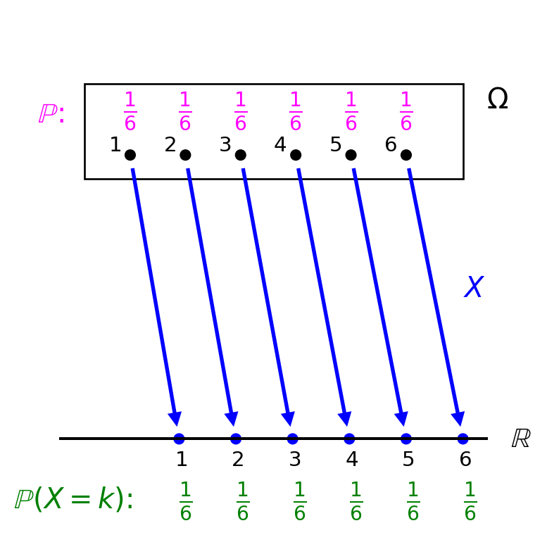
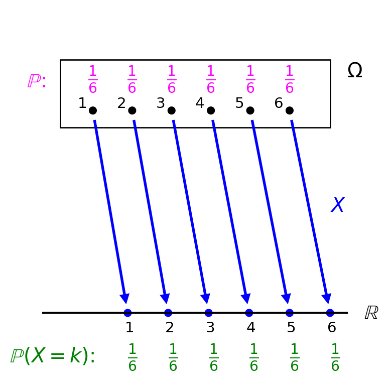
Example 4.1 Nothing like an easy example worked out in detail to alleviate any worries you may have. Consider the boring but hence easy to understand case where $X$ represents the outcome of rolling a die, so that we can for instance take $\Omega=\{1,\ldots,6\}$, $\mathcal{F}=\mathcal{P}(\Omega)$, $\P$ is determined by the values it assigns to the singletons i.e. $\P(\{1\})=\ldots=\P(\{6\})=1/6$, and we can simply set $X: \Omega \to \R$ equal to the identity i.e. $X(\omega)=\omega$ for all $\omega \in \Omega$. We’ve seen this all before, in Example 2.2 for instance.

Let’s take the event $C$ that the outcome is larger than $3$ i.e. $C=\{4,5,6\}$.

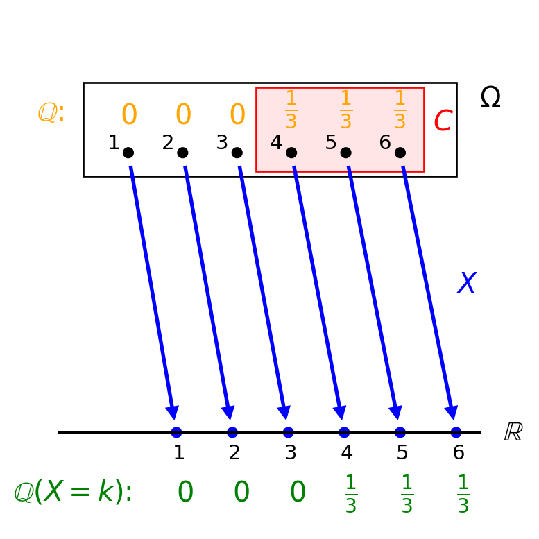
Let’s first argue by intuition what happens if we condition on $C$ i.e. assume that the event happens. As mentioned in Section 4.2, ultimately the effect of conditioning is that the probability measure $\P$ gets replaced by a new one. Let’s call it $\Q$. Conditional on $C$, the outcomes $1$, $2$ and $3$ are no longer possible and hence get probability $0$. The outcomes in $C$ remain equally likely, and since they should add up to $1$ they should all get probability $1/3$. In conclusion, our new probability measure should be given by $\Q(\{1\})=\Q(\{2\})=\Q(\{3\})=0$ and $\Q(\{4\})=\Q(\{5\})=\Q(\{6\})=1/3$.

If our intuition is right that this $\Q$ indeed describes the probabilies we get if we start with $\P$ and then condition on $C$, then it should be the case that \[\Q(A)=\P(A \, | \, C) \quad \text{for any event $A$}\] (this is in maths exactly what the previous sentence is trying to say). If we take for instance $A=\{5,6\}$ then on the one hand, using our def of $\Q$ and countable additivity (cf. Definition 1.3) \[\Q(A)=\Q(\{5\})+\Q(\{6\})=\frac{2}{3}\] while on the other hand, using Definition 4.1 i and again countable additivity \[\P(A \, | \, C)=\frac{\P(\{5,6\} \cap \{4,5,6\})}{\P(\{4,5,6\})}=\frac{\P(\{5,6\})}{\P(\{4,5,6\})}=\frac{2/6}{3/6}=\frac{2}{3}.\] So that’s a check!

Next let’s look at the distribution of $X$. Since $X$ is discrete, we can simply (literally) look at the values that $X$ takes in $\R$ i.e. its range and corresponding probabilities (as opposed to the more general and elaborate cdf and/or measure $\mu_X$ from Section 2.5). In the original situation i.e. without conditioning, the range is $\{1,\ldots,6\}$ with probabilities $\P(X=k)=1/6$ for $k=1,\ldots,6$. So using the well known summation formula for expectation of a discrete random variable (recall from Proposition 3.5 i) we get the well known result \[\E[X]=\sum_{k=1}^6 k \P(X=k)=\frac{1}{6} (1+2+\ldots+6)=\frac{7}{2}.\]

With the conditioning in force, first using our intuitively derived new probability measure $\Q$ (recall: nothing changes about the mapping $X$ i.e. it remains the identity mapping and its range remains $\{1,\ldots,6\}$) tells us that the expectation of $X$ changes to \[\E_{\Q}[X]=\sum_{k=1}^6 k \, \Q(X=k)=\frac{1}{3} (4+5+6)=5\] (this “$\E_{\Q}$” is commonly used notation to indicate that the expectation is computed under the prob measure $\Q$). If we have done things right, then our official defintion of the expectation of $X$ conditional on $C$ i.e. $\E[X \, | \, C]$ should also result in $5$. For this, using Definition 4.1 ii, first observe that $\mathbf{1}_C X$ is the following random variable: \[\mathbf{1}_C(\omega) X(\omega)=\begin{cases} 0 & \text{if $\omega \in \{1,2,3\}$} \\ \omega & \text{if $\omega \in \{4,5,6\}$} \end{cases} \] and hence, again using the summation formula, \[\E[\mathbf{1}_C X]=0 \cdot \frac{3}{6}+4 \cdot \frac{1}{6}+5 \cdot \frac{1}{6}+6 \cdot \frac{1}{6}=\frac{15}{6}.\] So Definition 4.1 ii yields \[\E[X \, | \, C] = \frac{\E[\mathbf{1}_C X]}{\P(C)}=\frac{15/6}{1/2}=5,\] another check! :).

Finally, let’s see the law of total probability (cf. Exercise 4.4) in action. If we consider in addition to $C$ the event $C^c=\{1,2,3\}$ then together they make a nice partition of $\Omega$. Analogue to above you can compute the expectation of $X$ conditional on $C^c$: \[\E[X \, | \, C^c] = \frac{\E[\mathbf{1}_{C^c} X]}{\P(C^c)} = \frac{1 \cdot 1/6 + 2 \cdot 1/6 + 3 \cdot 1/6 + 0 \cdot 3/6}{1/2}=2,\] and according to the law of total probability it should hold that \[\E[X]=\E[X \, | \, C] \P(C) + \E[X \, | \, C^c] \P(C^c).\] We’ve seen already that $\E[X]=7/2$, and plugging stuff in the right hand side gives $5 \cdot 1/2 + 2 \cdot 1/2=7/2$ — third and final check!

In conclusion, there’s two points to this example. Firstly, just some basic working with the concepts from Definition 4.1 for you to check your understanding against. Secondly, it shows that our alternative, intuitive way of thinking via an alternative probability measure $\Q$ also works. Effectively, we give all outcomes outside $C$ new probability $0$ while all outcomes in $C$ a new probability that is their old one but properly scaled up so that the new probability of $C$ becomes $1$. In more general terms, it is nothing but the “zooming in” procedure from the universe/outcome space $\Omega$ to the smaller universe/outcome space $C$ as already described in Exercise 1.3, with as probability measure on this new universe/outcome space the old one but properly scaled up. For a visual, see Figure 4.1 below.

(a) Without any conditioning. In magenta the probabilities $\mathbb{P}$ assigns to the possible outcomes, and in green the distribution of $X$ that results in

Exercises

You can now do Exercise 4.2–Exercise 4.5.

4.4 Conditioning on a sigma-algebra

Now let’s move on from conditioning on an event to conditioning on a $\sigma$-algebra. I’m guessing that this will be new for many of you. We’ll do this in three steps: first create some more feel for what you can do with partitions of $\Omega$, next we’ll look at conditioning on a finite $\sigma$-algebra (where these partitions come in very handy), and finally we’ll move on to the full blown general definition. Recall that the goal is still to compute the expectation of $X$ (or: the “best representation” of $X$) with this conditioning in force (whatever that exactly means!). The first two steps rely heavily on the stuff from the above Section 4.3, so do make sure to have a read through that one even if you’re quite familiar with conditioning on an event!

First for the partitions feel. Consider again the BBQ example where each possible outcome $\omega \in \Omega$ is a list of people that end up attending, and $X: \Omega \to \R$ gives the number of sausages you end up needing depending on the outcome. Consider also again the three events $C_1$: only vegetarians attend, $C_2$: at least 1 but at most 5 sausage eaters attend, and $C_3$: 6 or more sausage eaters attend, which form a partition of the outcome space $\Omega$.

Without any extra information, your best prediction for $X$ is simply its expectation $\E[X]$ (cf. Remark 4.1). Now suppose that you have a slightly mysterious neighbour who is into black arts and things, and he sees you the evening before your BBQ struggling with your decision making. Suppose that the neighbour tells you that he will have a go with his tarrot cards and that the next morning, not long before the BBQ starts, he will be able to tell you which of the three events $C_1$, $C_2$ or $C_3$ will happen (as it’s a partition, it’s guaranteed to be exactly one of them), and let’s assume that he is reliable ;). How would this affect your decision about the number of sausages to get, which currently stands at $\E[X]$?

Well you’d prepare the evening before by computing how many sausages you want to get in each scenario no. If the next morning he tells you it will be $C_1$, then your uncertainty is narrowed down to that event only, yet on the other hand you still don’t exactly know how many sausages you’ll need of course. In that scenario, your best prediction for $X$ would become the “average value” of $X$ on $C_1$ i.e., as dicussed in Section 4.3, $\E[X \, | \, C_1]$. Say that it equals $0$. Similarly, if he tells you $C_2$ or $C_3$, then your best prediction for $X$ becomes $\E[X \, | \, C_2]$ (say it equals $8$) or $\E[X \, | \, C_3]$ (say it equals $24$). You can compute all of that the evening before. And then the next morning, when the nighbour tells you his prediction, you quickly run to the shop to get either $0$ (maybe then you don’t have to go I guess!), $8$ or $24$ sausages.

So where does this leave you, the evening before the BBQ? Effectively with a best prediction for $X$ that is no longer $\E[X]$ but has turned into the following: \[\text{best prediction for $X$}=\begin{cases} \E[X \, | \, C_1]=0 & \text{if $C_1$ happens} \\ \E[X \, | \, C_2]=8 & \text{if $C_2$ happens} \\ \E[X \, | \, C_3]=24 & \text{if $C_3$ happens.} \end{cases} \] If you stare at this for a bit, realising that $C_i$ happens if and only if the outcome of the experiment i.e. people showing up $\omega$ is an element of it (and reminding ourselves $C_1, C_2, C_3$ form a partition), this is actually nothing but a random variable $Z: \Omega \to \R$ given by \[Z(\omega)=\begin{cases} \E[X \, | \, C_1] & \text{if $\omega \in C_1$} \\ \E[X \, | \, C_2] & \text{if $\omega \in C_2$} \\ \E[X \, | \, C_3] & \text{if $\omega \in C_3$} \end{cases} = \begin{cases} 0 & \text{if $\omega \in C_1$} \\ 8 & \text{if $\omega \in C_2$} \\ 24 & \text{if $\omega \in C_3$.} \end{cases} \tag{4.5}\] This is, as we will see in a sec, the essence of what conditioning on a $\sigma$-algebra is — even though we haven’t even used the word “$\sigma$-algebra” yet!

Let me add a little bend to this story. Do you actually really need your neighbour for this? No, well at least not to determine this random variable $Z$ right, that’s all your own work. Maybe this neighbour was a figment of your imagination in the first place, I mean, a neighbour who can reliably predict the future? Come on, really? Are you sure you didn’t have a bit too much of the beer already that you got for the BBQ? The prediction story is one (viable) interpretation for $Z$, but $Z$ as defined in Equation 4.5 is of course just a mathematical object that you can interpret however you like.

You can also think about $Z$ as a simplified representation of $X$: where $X$ is a random variable that (potentially) takes a different value for every $\omega \in \Omega$, $Z$ has only three different possible values. You create $Z$ by first choosing $C_1$, $C_2$ and $C_3$, and then, on each $C_i$, squashing the different values that $X$ (potentially) takes down to a single number (its “average value”). It is, given the choice for $C_1, C_2, C_3$, the best simplified representation of $X$, in the following sense: in the class of all random variables that are constant on $C_1, C_2, C_3$ i.e. any $Y$ of the form \[Y(\omega)=\begin{cases} a & \text{if $\omega \in C_1$} \\ b & \text{if $\omega \in C_2$} \\ c & \text{if $\omega \in C_3$} \end{cases} \] for any $a,b,c \in \R$, $Z$ as defined in Equation 4.5 is closest to $X$ under the mean squared error as introduced in Remark 4.1. We’ll be slightly more precise about this after the general definition.

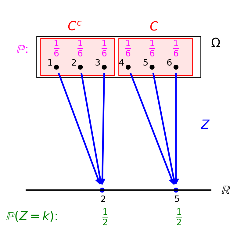
Example 4.2 Consider our good old rolling the die example from Example 4.1 again. As already discussed there, one example of a partition of $\Omega$ are the events $C=\{4,5,6\}$ and $C^c=\{1,2,3\}$, with $\E[X \, | \, C]=5$ and $\E[X \, | \, C^c]=2$, and $\P(C)=\P(C^c)=1/2$. Based on this partition, the analogue of Equation 4.5 in this case hence boils down to \[Z(\omega)=\begin{cases} 2 & \text{if $\omega \in C^c$} \\ 5 & \text{if $\omega \in C$.} \end{cases} \tag{4.6}\] See Figure 4.2 for a visual.

(a) The original situation as in Figure 4.2 (a)

Now let’s move on to the next steps: actually talking about $\sigma$-algebras. Before we do that, let’s discuss one particularly useful way of looking at/interpreting $\sigma$-algebras:

Remark 4.3. On some outcome space $\Omega$, we can interpret a $\sigma$-algebra as representing a certain level of information (about the outcome of the experiment), as follows.

Take a $\sigma$-algebra $\mathcal{F}$ on $\Omega$. If the experiment is performed with a certain outcome $\omega$, then a number of events in $\mathcal{F}$ happen (always at least one since every $\sigma$-algebra contains $\Omega$), namely the ones containing $\omega$, and a number won’t, namely the ones not containing $\omega$. You can look at that the other way around: if you know which events in a $\sigma$-algebra happen, how much information does that provide about what the outcome exactly was? For example:

The $\sigma$-algebra $\{\emptyset,\Omega\}$ provides no information at all: each time the experiment is performed, $\emptyset$ doesn’t happen and $\Omega$ does happen. That doesn’t tell you anything about what the oucome actually was.
The powerset $\mathcal{P}(\Omega)$ (which, recall, contains all possible subsets of $\Omega$) provides the highest level of information: since it contains all subsets, it also contains all singletons $\{\omega\}$ for all $\omega \in \Omega$. So each time the experiment is performed, you can simply look at these singletons: see which one happens and you know exactly what the outcome of the experiment was.

In general, intuitively at least (uncountability and things), by taking the intersection of all elements in the $\sigma$-algebra that happen you get the smallest event that you know happens, and the level of info that this $\sigma$-algebra provides is the statement “the outcome must be an element from this [smallest event]”. Obviously, the smaller the [smallest event] is the more informative it is (with the [smallest event] always being a singleton, like is the case for the powerset, as most optimal case).

Here are a few consequences of this perspective:

If $\mathcal{G}$ is a sub-$\sigma$-algebra of $\mathcal{F}$ i.e. $\mathcal{G} \subseteq \mathcal{F}$ then $\mathcal{G}$ provides a lower (weakly speaking: either equal or strictly lower) level of information than $\mathcal{F}$ (for any outcome $\omega$). Indeed because every event in $\mathcal{G}$ is also in $\mathcal{F}$, whatever [smallest event] $\mathcal{G}$ manages to produce, $\mathcal{F}$ will be able to produce that one as well and potentially even something that is strictly smaller.

In this context people often say that $\mathcal{G}$ is coarser than $\mathcal{F}$ resp. $\mathcal{F}$ finer than $\mathcal{G}$.
If a random variable $X$ is $\mathcal{F}$-measurable (cf. Definition 2.1) then the level of information that $\mathcal{F}$ provides is enough to deduce the value that $X$ takes, i.e. if the experiment is executed with (unseen) outcome $\omega$, to deduce what $X(\omega)$ is. To convince yourself, observe that $\mathcal{F}$ contains for instance all events of the form $X^{-1}((-\infty,x])$ for $x \in \R$ and that the ones that will happen are exactly all the ones so that $x \geq X(\omega)$.
If $\mathcal{G}$ is a finite $\sigma$-algebra, then we know from Example 1.4 that it has a nice and convenient structure: it contains atoms $C_1, \ldots, C_n$ that make up its smallest elements, in the sense that other than $\emptyset$ each element in $\mathcal{G}$ is a union of one or more of these $C_i$’s. That means that this [smallest event] mentioned above will always be exactly one of these $C_i$’s. So the level of information this $\sigma$-algebra provides is which one of the $C_i$’s happens.

This view of $\sigma$-algebras is not only useful here but will also be prominent when we talk about filtrations later on in the course!

Back to the main storyline: on some probability space $(\Omega,\mathcal{F},\P)$ where an integrable random variable $X$ lives (i.e. $\E[|X|]<\infty$), let $\mathcal{G} \subseteq \mathcal{F}$ be a sub-$\sigma$-algebra of $\mathcal{F}$. For the second in our three step programme, assume that $\mathcal{G}$ is finite.

Let $C_1, \ldots, C_n$ be the atoms of $\mathcal{G}$ (as reiterated in the above Remark 4.3), and assume for the moment that $\P(C_i)>0$ for all $i=1,\ldots,n$. Consider the analogue simplified representation of $X$, as in Equation 4.5: on each $C_i$, compute the number $\E[X \, | \, C_i]$ (which is well defined since $\P(C_i)>0$) and create a random variable $Z: \Omega \to \R$ by setting it equal to $\E[X \, | \, C_i]$ on $C_i$ for all $i=1,\ldots,n$: \[Z(\omega)=\begin{cases} \E[X \, | \, C_1] & \text{if $\omega \in C_1$} \\ \E[X \, | \, C_2] & \text{if $\omega \in C_2$} \\ \qquad \vdots & \qquad \vdots \\ \E[X \, | \, C_n] & \text{if $\omega \in C_n$} \end{cases} = \sum_{i=1}^n \E[X \, | \, C_i] \mathbf{1}_{C_i}(\omega) \tag{4.7}\] (note that the second expression is just a more compact version that is trivially the same thing as you can easily check, we also used it in Section 3.3.1 e.g.).

Analogue to the BBQ example, $Z$ represents your best prediction for the value of $X$ if it will be revealed to you which events in $\mathcal{G}$ happen (or, equivalently as discussed in Remark 4.3, which event $C_i$ will happen); “best” in the sense that among all $\mathcal{G}$-measurable random variables i.e. all random variables of the form \[Y(\omega)=\begin{cases} a_1 & \text{if $\omega \in C_1$} \\ a_2 & \text{if $\omega \in C_2$} \\ \ \vdots & \qquad \vdots \\ a_n & \text{if $\omega \in C_n$} \end{cases} \tag{4.8}\] for any real numbers $a_1, \ldots, a_n$, it is the one that is closest (think: “most alike”) to $X$ under the mean squared error (again, we’ll be a bit more precise after the general definition).

Note that $Z$ is truely a simplified representation of $X$: given $X$ you can deduce $Z$ (by Equation 4.7) but vice versa, given $Z$ you can generally not recover what $X$ was (since on each $C_i$ you only know the “average value” of $X$, not what the individual values $X(\omega)$ for $\omega \in C_i$ were). This ties in very nicely with the “$\sigma$-algebra as level of information” perspective in Remark 4.3, combining the first two bullet points there: any $\mathcal{G}$-measurable random variable is also $\mathcal{F}$-measurable but not necessarily the other way around, since $\mathcal{F}$ provides a higher level of information than $\mathcal{G}$ it can accommodate, roughly speaking, more intricate random variables than $\mathcal{G}$ can. So by “projecting” the $\mathcal{F}$-measurable random variable $X$ onto $\mathcal{G}$, resulting in the $\mathcal{G}$-measurable random variable $Z$, we “lose information” — unless $X$ is also $\mathcal{G}$-measurable i.e. $\mathcal{G}$ is also able to accommodate $X$, in which case $Z=X$.

We call this $Z$ the conditional expectation of $X$ given the $\sigma$-algebra $\mathcal{G}$. We’ll give $Z$ some special notation later. Let’s wrap up the one loose end: what do we do if one or more $C_i$’s have probability $0$ so that corresponding $\E[X \, | \, C_i]$’s are not defined? Basically we don’t care about those: just give $Z$ some arbitrary value, say $0$, on any of these. This may seem strange, but note that the union of such $C_i$’s also has probability $0$ (e.g. using subadditivity, cf. Theorem 1.1 iii) and as we will see in the general definition, we won’t care a lot about probability $0$ events.

We’re close to the general definition now! Before we can move on to the final third step, let’s get to know this $Z$ a little bit better by discussing some of its properties:

$Z$ is $\mathcal{G}$-measurable. In fact more precisely a random variable $Y$ is $\mathcal{G}$-measurable if and only if it is of the form Equation 4.8.

To prove this, for the “if” direction, we have already seen this in Exercise 2.3.

For the “only if” direction, if $Y$ is $\mathcal{G}$-measurable then by def (Definition 2.1), $Y^{-1}((-\infty,x]) \in \mathcal{G}$ for all $x \in \R$. Now consider what happens to $Y^{-1}((-\infty,x])$ as you start with $x$ near $-\infty$ and let it increase towards $\infty$. Because the interval $(-\infty,x]$ grows, the inverse image $Y^{-1}((-\infty,x]) \in \mathcal{G}$ either stays the same or gets larger. Since $\mathcal{G}$ has only finitely many elements, the inverse image $Y^{-1}((-\infty,x]) \in \mathcal{G}$ can only become strictly larger finitely often, say as we cross the points $x_1, x_2, \ldots, x_m$. Because each element in $\mathcal{G}$ (other than $\emptyset$) is a union of one or more of the $C_i$’s, each time we cross such a point $x_j$ and $Y^{-1}((-\infty,x])$ becomes larger, it must be because one or more of the $C_i$’s are added to it. The fact that the ones that are added are present in $Y^{-1}((-\infty,x_j])$ but not in $Y^{-1}((-\infty,x])$ for $x<x_j$ means that for any $\omega$ in the ones that are added, $Y(\omega)=x_j$. Ultimately, for $x>x_m$, each $C_1, \ldots, C_n$ has been added at some point in this process, and in particular it shows that $Y$ is constant on each $C_i$ i.e. of the from Equation 4.8.
For any $A \in \mathcal{G}$ we have that $\E[\mathbf{1}_A Z]=\E[\mathbf{1}_A X]$. To see this, first consider $A=C_i$ for some $i=1,\ldots,n$. Observe that by very def (cf. Equation 4.7) we have the pointwise identity \[\mathbf{1}_{C_i} Z=\mathbf{1}_{C_i} \E[X \, | \, C_i]\] and so indeed \[\E \left[ \mathbf{1}_{C_i} Z \right] = \E \left[ \mathbf{1}_{C_i} \E[X \, | \, C_i] \right] = \E[X \, | \, C_i] \E \left[ \mathbf{1}_{C_i} \right] = \E[X \, | \, C_i] \P(C_i) = \E \left[ \mathbf{1}_{C_i} X \right],\] where the second equality uses linearity (cf. Proposition 3.6 i, after all $\E[X \, | \, C_i]$ is just a number!), and the final equality uses the def of $\E[X \, | \, C_i]$ (cf. Definition 4.1 ii).

Any other $A \in \mathcal{G}$ is either $\emptyset$ in which case both sides equal $0$, or the union of two or more of the $C_i$’s. However since the $C_i$’s are disjoint, the indicator function of $A$ is just the sum of indicator functions of two or more of the $C_i$’s (cf. Exercise 4.2) and hence by linearity, the result follows from the fact that it holds for each $C_i$ as seen above.

Interpretation wise, this property expresses the level of similarity between $Z$ and $X$: even though they are (generally) different random random variables, this property shows in what way they are alike each other. Note that setting $A=\Omega$, we have in particular also that $\E[Z]=\E[X]$.

Example 4.3 One more time back to the die example in Example 4.1 & Example 4.2. Recalling the event $C=\{4,5,6\}$, consider $\mathcal{G}=\left\{ \emptyset, C, C^c, \Omega \right\}$ (one of our favourite simple $\sigma$-algebras, see e.g. Example 1.3). The atoms of this $\mathcal{G}$ are (of course) $C$ and $C^c$.

Given the work already done in Example 4.2, we can now officially say that the random variable $Z$ defined in Equation 4.6 is the conditional expectation of $X$ given $\mathcal{G}$!

Ok, time for the final step three in our master plan now! Recall the setting: a probability space $(\Omega,\mathcal{F},\P)$ with an integrable random variable $X$ and a sub-$\sigma$-algebra $\mathcal{G} \subseteq \mathcal{F}$, where we now drop the assumption that $\mathcal{G}$ is finite.

Having seen the above natural and elegant stuff for the case of a finite $\sigma$-algebra, can we somehow still make sense of a conditional expectation of $X$ on a (more) general $\mathcal{G}$ as well?? The problem is of course that our intuition & construction from above no longer works: a general $\mathcal{G}$ does not necessarily have nice/non-trivial “smallest” elements making up a finite partition of $\Omega$, which was core to our reasoning above.

A way forward here is a commonly employed strategy in such a situation: even if the construction/(initial) intuiton no longer works, can we go “top down” rather i.e. can we identify some properties of the object we constructed (in this case $Z$ from Equation 4.7) that we consider fundamental/characteristic, and can we try to establish whether an object with these characteristics still exists? In this case, it turns that the right properties to use as characteristics are the ones appearing in the two bullet points above. And the good news is that the answer is “yes, also in the general case a random variable $Z$ with these characteristics still exists”. The (slightly) bad news is that there is no unique choice — although at least any two possible choices are a.s. equal:

Definition 4.2 On a probability space $(\Omega,\mathcal{F},\P)$, let $X$ be an integrable (i.e. $\E[|X|]<\infty$, cf. Definition 3.4) random variable and let $\mathcal{G}$ be a sub-$\sigma$-algebra of $\mathcal{F}$ i.e. $\mathcal{G} \subseteq \mathcal{F}$. Then there exists an integrable random variable $Z$ with the properties:

$Z$ is $\mathcal{G}$-measurable,
for any event $A \in \mathcal{G}$ it holds that $\E[\mathbf{1}_A Z]=\E[\mathbf{1}_A X]$.

If $\widetilde{Z}$ is any other random variable satisying properties i and ii, then $\widetilde{Z}=Z$ a.s. (i.e. $\P(\widetilde{Z}=Z)=1$, cf. Section 2.4).

We call any $Z$ satisfying these two properties (a version of) the conditional expectation of $X$ given the $\sigma$-algebra $\mathcal{G}$ and denote it by $\E[X \, | \, \mathcal{G}]$.

If $\mathcal{G}$ is finite with atoms $C_1,\ldots,C_n$ (cf. Example 1.4) with $\P(C_i)>0$ for all $i=1,\ldots,n$, then we can (and normally will) make the explicit choice \[Z(\omega)=\E[X \, | \, \mathcal{G}](\omega)=\begin{cases} \E[X \, | \, C_1] & \text{if $\omega \in C_1$} \\ \E[X \, | \, C_2] & \text{if $\omega \in C_2$} \\ \qquad \vdots & \qquad \vdots \\ \E[X \, | \, C_n] & \text{if $\omega \in C_n$} \end{cases} = \sum_{i=1}^n \E[X \, | \, C_i] \mathbf{1}_{C_i}(\omega). \tag{4.9}\]

Intuitively (at least) we can interpret $\E[X \, | \, \mathcal{G}]$ as a simplified representation of $X$, that is the best prediction of $X$ if it will be revealed to you which events in $\mathcal{G}$ happen, and is within the class of all $\mathcal{G}$-measurable random variables the one that is closest to/most alike $X$.

Some notes:

For a proof of the existence of a random variable satisfying properties i and ii (if $\mathcal{G}$ is not finite), see e.g. Section 9.2 in Williams (1991). See also Section 4.7.2 for an alternative construction. For the almost sure uniqueness, see Exercise 4.8.
If we restrict ourselves to random variables with finite second moments, the above “closest to/most alike” statement can be made precise and proven, see Exercise 4.12.
Despite having “expectation” in its name and the symbol containing an “$\E$”, this conditional expectation is (generally) a random variable rather than a number! Think about “$\E[X \, | \, \mathcal{G}]$” as just an elaborate name for a random variable where we otherwise would use just a “$Y$” or “$Z$” or so — of course this name does carry the information what the original random variable is ($X$) and what $\sigma$-algebra we’re conditioning on ($\mathcal{G}$).
The fact that we do not (pointwise) uniquely define this conditional expectation may seem problematic at first. But then, you are actually already quite well used to such a concept: for continuous random variables the pdf is also not uniquely defined (recall Remark 2.6), yet nevertheless you’re happily working with pdf’s for years already without getting into trouble with this. The reason is that the (primary) way in which you use pdf’s is integrating them to compute probs/expectations, and for that purpose it doesn’t matter which of the many possible pdf’s for the given random variable in question you use.

Similarly, for our intended purposes of this conditional expectation this non-uniqueness doesn’t matter: any statements/results/operations etc. will be valid no matter which “version” of $\E[X \, | \, \mathcal{G}]$ we exactly use. We will generally just talk about the conditional expectation, although that is strictly speaking incorrect in the same way that talking about the pdf of a continuous random variable is.

This does have the ramification that any statement/result of a form like “$\E[X \, | \, \mathcal{G}]=...$” can only ever be true almost surely “at most”, not pointwise. Going forward, where particularly relevant we’ll try to point this out but it’s of course very good to make this a standard part of your understanding as well!
If $\mathcal{G}$ is finite but one or more of its atoms have probability $0$, then you can still make Equation 4.9 work: just set $Z(\omega)$ in Equation 4.9 equal to some arbitrary value if $\omega$ is an element of any such atom. You can check that this $Z$ still satisfies properties i and ii. The fact that Equation 4.9 now no longer uniquely defines $Z$ but that on the other hand any two choices only differ on a set of probability $0$ is just a manifestation of the previous bullet point!

Remark 4.4. Now that we have put all the pieces together and have a full definition, we could summarise the interpretation of the “prediction” purpose of conditional expectations as follows (generalising the reasoning from the earlier BBQ-with-magical-neighbour example). On some probability space $(\Omega,\mathcal{F},\P)$ with integrable random variable $X$ and sub-$\sigma$-algebra $\mathcal{G}$:

you determine the random variable $\E[X \, | \, \mathcal{G}]$ using Definition 4.2,
the experiment is done and the outcome is an $\omega \in \Omega$ (unknown to you),
you are being told which events in $\mathcal{G}$ happen (i.e. which ones contain $\omega$),
on the basis of the information in 2 only you can compute the number $\E[X \, | \, \mathcal{G}](\omega) \in \R$ (cf. Remark 4.3)
your best prediction for the unknown value of $X(\omega)$ is your $\E[X \, | \, \mathcal{G}](\omega)$.

Note that step 0 has to be done only once, after which steps 1–4 can be repeated as often as you like (with typically a different outcome $\omega$ each time).

In this section I have tried to guide you to this definition & interpretation in a way that I hope makes it accessible for all of you. As you’ll probably have realised while reading it, there are multiple ways/angles from which you can look at this object. Of course, by all means make your own choices and build your own favourite perspective!

Exercises

You can now do Exercise 4.6–Exercise 4.8.

4.4.1 Conditional (on a sigma-algebra) probabilities

We discussed in Section 4.3 how, in the context of conditioning on an event, you could see the definition of the conditional probability just as a consequence of the definition of conditional expecation of a random variable by plugging indicator functions into the latter. Now that we have established conditioning on $\sigma$-algebras for random variables, it is tempting to explore whether that principle could be applied here as well.

That is to say, on some probability space $(\Omega,\mathcal{F},\P)$ and with $\mathcal{G}$ be a sub-$\sigma$-algebra of $\mathcal{F}$, we could (and do) define for events $A \in \mathcal{F}$ the conditional probability of $A$ given the $\sigma$-algebra $\mathcal{G}$ as \[\P(A \, | \, \mathcal{G}) := \E \left[ \mathbf{1}_A \, | \, \mathcal{G} \right]. \tag{4.10}\] Now, keep in mind that since the right hand side, as defined in Definition 4.2, is a random variable (rather than a number), and hence so is the left hand side, which stretches our understanding of what a probability means a bit. Nevertheless we could take this at face value and investigate some of its properties. First note that (using Exercise 4.6) \[\P(\emptyset \, | \, \mathcal{G})=\E \left[ \mathbf{1}_\emptyset \, | \, \mathcal{G} \right]=\E \left[ 0 \, | \, \mathcal{G} \right]=0 \quad \text{(a.s.)}\] and similarly $\P(\Omega \, | \, \mathcal{G})=1$ (a.s.). Further there’s even countable additivity: if $A_1, A_2, \ldots \in \mathcal{F}$ are mutually disjoint events, then we have a.s. \[\begin{aligned} \P \left( \bigcup_{i=1}^\infty A_i \right) &= \E \left[ \left. \mathbf{1}_{\bigcup_{i=1}^\infty A_i} \, \right| \, \mathcal{G} \right] \\ &= \E \left[ \left. \sum_{i=1}^\infty \mathbf{1}_{A_i} \, \right| \, \mathcal{G} \right] \\ &= \sum_{i=1}^\infty \E \left[ \mathbf{1}_{A_i} \, | \, \mathcal{G} \right] \\ &= \sum_{i=1}^\infty \P(A_i \, | \, \mathcal{G}), \end{aligned} \] where the second equality uses a slight extension (proven in the same way) of Exercise 4.2 and the third uses the Monotone Convergence Theorem for conditional expectations which we’ll encounter in Section 4.6. So these properties seem very nicely in line with how we need a probability measure to behave (cf. Definition 1.3)!

However, there are obvious problems with trying to see this as a probability measure as well: these “a.s.”’s i.e. “almost surely”’s everywhere. For starters, since the right hand side in Equation 4.10 is not pointwise uniquely defined, neither is the left hand side. So we can’t really talk about this object as a mapping $A \mapsto \P(A \, | \, \mathcal{G})$ withour further ado, because any mapping should assign a single, well defined value (whatever object it may be) to all of its arguments.

What we effectively need to resolve this problem (don’t worry about this for exam purposes), is a process to identify for each event $A$ the version of the conditional expectation $\E [ \mathbf{1}_A \, | \, \mathcal{G} ]$ that we want to use, in a consistent way throughout the above. That is, a mapping $\mathbf{P}: \Omega \times \mathcal{F} \to [0,1]$ so that

for any event $A \in \mathcal{F}$, the random variable $Y$ given by $Y(\omega)=\mathbf{P}(\omega,A)$ is a version of $\E [ \mathbf{1}_A \, | \, \mathcal{G} ]$, and
there exists an almost sure event $\Omega_0 \in \mathcal{F}$ so that for every $\omega \in \Omega_0$ fixed, the mapping $A \mapsto \mathbf{P}(\omega,A)$ for $A \in \mathcal{F}$ is a probability measure on $(\Omega,\mathcal{F})$ (in the usual sense of Definition 1.3).

If such a mapping $\mathbf{P}$ exists, then we call it a regular conditional probability given the $\sigma$-algebra $\mathcal{G}$ and we can use for $A \in \mathcal{F}$ (pointwise) \[\P(A \, | \, \mathcal{G})(\omega)=\mathbf{P}(\omega,A),\] i.e. this is our particular choice from all versions of $\E [ \mathbf{1}_A \, | \, \mathcal{G} ]$. It’s beyond the scope of this course to say a lot more about this, let’s conclude with saying that such regularity exists on “most” probability spaces (especially the ones we tend to naturally use) but not on every probability space. If you’re interested in more details, see e.g. Section 9.9 in Williams (1991) and Chapter 6 in Kallenberg (1997).

4.5 Conditioning on a random variable

The final specific form of conditioning to discuss is that of conditioning on a random variable $Y$. You’ll most likely have already encountered this in earlier probability courses, but now we have available the context of conditioning on a $\sigma$-algebra we can discuss that conditioning on a random variable is nothing but a special case!

On some probability space $(\Omega,\mathcal{F},\P)$, let $Y$ be a random variable. Recall from Definition 2.2 that it naturally generates a $\sigma$-algebra denoted by $\sigma(Y)$, which is just the collection of inverse images $Y^{-1}(B)=\{Y \in B\}$ for all Borel sets $B$. It is the smallest $\sigma$-algebra that makes $Y$ measurable (by very def, cf. Definition 2.1), and since $Y$ is $\mathcal{F}$-measurable (being a random variable) it must be the case that $\sigma(Y) \subseteq \mathcal{F}$. So for any (other) random variable $X$ on this probability space, we can use the machinery from Section 4.4 to consider $X$ conditioned on $\sigma(Y)$. For convenience of notation, and in keeping with already existing notation from earlier probability courses, we tend to write \[\E[X \, | \, Y] := \E[X \, | \, \sigma(Y)]\] and similarly for events $A \in \mathcal{F}$ \[\P(A \, | \, Y):=\P(A \, | \, \sigma(Y)).\]

As discussed in Section 4.4, conditioning on $\sigma(Y)$ means that we consider $X$ (or $A$) under the extra information that we will be told which events in $\sigma(Y)$ happen or, equivalently, that we will be told which value $Y$ takes. This formulation is probably how conditioning on a random variable was motivated/introduced to you in earlier probability courses! In this spirit, we should expect the random variable $\E[X \, | \, Y]$ to be, roughly speaking, a list of values: one for each possible value that $Y$ can take i.e. in the range of $Y$. Or, put slightly more generally, that $\E[X \, | \, Y]$ is some function of $Y$.

Indeed, in the case that $Y$ is a discrete random variable with range $\{y_1,\ldots,y_n\}$, it is not hard to convince yourself that $\sigma(Y)$ is a finite $\sigma$-algebra with atoms (cf. Example 1.4) $Y^{-1}(\{y_i\})=\{Y =y_i\}$ for $i=1,\ldots,n$. That means that we can apply Definition 4.2 where the $C_i$’s are exactly these inverse images to deduce that \[\E[X \, | \, Y](\omega)=\begin{cases} \E[X \, | \, Y=y_1] & \text{if $Y(\omega)=y_1$} \\ \E[X \, | \, Y=y_2] & \text{if $Y(\omega)=y_2$} \\ \qquad \vdots & \qquad \vdots \\ \E[X \, | \, Y=y_n] & \text{if $Y(\omega)=y_n$} \end{cases} = \sum_{i=1}^n \E[X \, | \, Y=y_i] \mathbf{1}_{\{Y=y_i\}}(\omega) \] which we can maybe more conveniently express as, where $R_Y$ denotes the range of $Y$: \[\E[X \, | \, Y]=\psi(Y), \text{ where } \psi:R_Y \to \R \text{ is given by } \psi(y)=\E[X \, | \, Y=y] \tag{4.11}\] (note that $\E[X \, | \, Y=y]$ is the expectation of $X$ conditional on the event $\{Y=y\}$ as discussed in Section 4.3).

Formula Equation 4.11 is one that probably rings a bell with you as seen in earlier probability courses, and indeed as the standard tool to evaluate $\E[X \, | \, Y]$: you work out what function $\psi$ is for the situation at hand from its def in Equation 4.11, and then write down what $\E[X \, | \, Y]=\psi(Y)$ boils down to. Recall for this purpose also the tools of conditional cdf’s/pmf’s/pdf’s to analyse (the distribution of, and hence expectation of) $X$ conditional on $Y=y$ as referred to in Remark 4.2.

However, as you’ll remember, you need to be careful with non-discrete $Y$ and values $y$ in their range with $\P(Y=y)=0$: in such a case $\E[X \, | \, Y=y]$ is after all not well defined. Even though we can’t make sense of conditioning on an event of probability $0$ in general (see e.g. the Borel–Kolmogorov paradox), as long as for any $\eps>0$ the event $\{Y \in (y-\eps,y+\eps)\}$ has strictly positive probability, $\E[X \, | \, Y=y]$ can be properly defined as the obvious limit. For instance in the case of a continuous $Y$, this is typically achieved by choosing a combination of pdf $f_Y$ (recall their non-uniqueness from Remark 2.6) and range $R_Y$⁴ so that $y \in R_Y$ if and only if $f_Y(y)>0$.

⁴ For any given mapping $Y:\Omega \to \R$, if you don’t like its range you could adjust it a little bit by redefining $Y(\omega)$ for $\omega$ in an event of probability $0$. The adjusted $Y$ has the same distribution as the original one (cf. Exercise 2.9) and is hence for computations like we’re doing here (“distributional” ones) indistinguishable from the original $Y$

4.6 Properties of conditional expectations (on sigma-algebras)

Of course, for doing useful stuff with conditioning (on a $\sigma$-algebra), only having the def Definition 4.2 is a bit bare bones, so the next stop is to discuss some properties. We’ll discuss the proof of some of them in this section, we’ll do some in the exercises, and for any remaining ones/more details see Section 9.7 in Williams (1991).

Just to reiterate: recall that a conditional expectation on a $\sigma$-algebra is a random variable (rather than a number) and recall that it is only defined up a.s. equivalence.

Let’s break them up in two categories. For the first category, even though this concept of a conditional expectation is not an expectation/integral in the literal sense as we discussed in Chapter 3, it does actually respect the fundamental properties an integral concept should have as outlined in Proposition 3.1 (properly reformulated) and consequently we can show many of the same properties (properly reformulated) we have previously encountered for expectations/integrals (cf. Theorem 3.1, Proposition 3.6, Theorem 3.2, Theorem 3.3):

Theorem 4.1 Let $(\Omega,\mathcal{F},\P)$ be a probability space on which integrable random variables $X, X_1, X_2, \ldots$ live, and let $\mathcal{G}$ be a sub-$\sigma$-algebra of $\mathcal{F}$. Then we have the following:

Linearity: for any $\alpha, \beta \in \R$, \[\E[\alpha X_1 + \beta X_2 \, | \, \mathcal{G}]=\alpha \E[X_1 \, | \, \mathcal{G}]+\beta \E[X_2 \, | \, \mathcal{G}] \quad \text{(a.s.).}\]
Non-negativity: if $X \geq 0$ a.s., then $\E[X \, | \, \mathcal{G}] \geq 0$ a.s.
Almost sure equivalence: $\E[|X| \, | \, \mathcal{G}] = 0$ a.s. if and only if $X=0$ a.s.
Jensen’s inequality: if $f: \R \to \R$ is convex (recall e.g. from Wiki) and $f(X)$ is integrable, then \[f \big( \E[X \, | \, \mathcal{G}] \big) \leq \E[f(X) \, | \, \mathcal{G}] \quad \text{(a.s.).}\]
Monotone convergence (MCT): if $0 \leq X_1 \leq X_2 \leq ...$ with (pointwise) limit $X$, then \[\lim_{n \to \infty} \E[X_n \, | \, \mathcal{G}] = \E[X \, | \, \mathcal{G}] \quad \text{(a.s.).}\]
Dominated convergence (DCT): if $X_n \stackrel{\text{a.s.}}{\longrightarrow} X$ as $n \to \infty$ and there exists an integrable random variable $Y$ so that for any $n=1,2,\ldots$ we have $\lvert X_n \rvert \leq Y$, then \[\lim_{n \to \infty} \E[X_n \, | \, \mathcal{G}] = \E[X \, | \, \mathcal{G}] \quad \text{(a.s.).}\]

Some notes:

Just to reiterate/clarify: all of these properties hold no matter what version of the relevant conditional expectations are being used. For instance, the linearity property states that if you take any version of $\E[X_1 \, | \, \mathcal{G}]$ and $\E[X_2 \, | \, \mathcal{G}]$, then $\alpha \E[X_1 \, | \, \mathcal{G}]+\beta \E[X_2 \, | \, \mathcal{G}]$ is a version of $\E[\alpha X_1 + \beta X_2 \, | \, \mathcal{G}]$ etc.
In the bigger picture of working/reasoning with such objects that are only defined almost surely, most of the time you won’t notice the difference with “normal” pointwise definitions, you can for instance in the usual way string together a sequence of (in)equalities where each step is almost surely true, and be certain that the almost sure (in)equality also holds between the ultimate left and right hand sides (this is just an application of Exercise 2.5).
Analogue to in Theorem 3.1 and Proposition 3.6, the non-negativity property together with linearity also implies that if $X_1 \leq X_2$ a.s. then $\E[X_1 \, | \, \mathcal{G}] \leq \E[X_2 \, | \, \mathcal{G}]$ a.s.

Note that linearity is obvious from Definition 4.2 since both conditions there survive linear combinations fine.

Before we carry on, let us first make a general statement as the proofs get a little bit more involved I think, especially also while you’re (likely) still need to get used somewhat to the “versions” issue with conditional expectations. When you’re embarking on proving something, always first make sure that you understand the statements fully. If needs be, go back to any definitions etc. to pick up on any objects etc. you’re not entirely sure about. Next give the statement a good stare in the face. Without thinking about proofs, does it make sense at face value? Why? What might make it fail? Have I seen something similar before, or do I remember a technique I could use to (partially) prove it? Pondering such things a bit helps gaining some insight, also in how you could structure a proof!

Ok, on to the non-negativity (property ii above). Does it make sense (in light of Definition 4.2)? Well if $X$ is non-negative, keeping in mind that taking an expectation preserves non-negativity (Proposition 3.6 ii), then yeah, it would make sense for condition ii of Definition 4.2 to carry non-negativity from $X$ over to $Z$/its conditional expectation no? So let’s try to use that connection in a proof. First note that since $X \geq 0$ a.s., for any event $A \in \mathcal{G}$ also $\mathbf{1}_A X \geq 0$ a.s. (because if $\mathbf{1}_A(\omega) X(\omega)<0$ then also $X(\omega)<0$ i.e. $\{ \mathbf{1}_A X < 0 \} \subseteq \{ X<0\}$). So Proposition 3.6 ii gives us that also $\E[\mathbf{1}_A X] \geq 0$. This means, writing $Z=\E[X \, | \, \mathcal{G}]$ (any version of it) for ease of notation, that from Definition 4.2 we also get that \[\E[\mathbf{1}_A Z] \geq 0 \quad \text{for all } A \in \mathcal{G}. \tag{4.12}\]

Now we need to somehow show that this also implies that $Z \geq 0$ a.s. Intuitively this makes sense, because if the event $\{Z<0\}$ had positive probability then it should surely be the case that $\E[\mathbf{1}_{\{Z<0\}} Z] < 0$ as well, because $\mathbf{1}_{\{Z<0\}}(\omega) Z(\omega)$ is either strictly negative (if $\omega \in \{Z<0\}$, an event with strictly positive probability which is hence “noticed” by $\E$, recall Remark 3.4) or $0$ right? That’s true, we just don’t have a result that nicely fits this and allows us to draw this conclusion without further ado. So we still need to do some work to make this precise. For this, assume that $\P(Z<0)>0$ and let’s hunt for a contradiction with Equation 4.12. Let’s use a technique we’ve encountered before, e.g. in Exercise 4.8, and is generally a very good one to keep in mind! The idea is that, if rather than the event $\{Z<0\}$ we would be looking at $\{Z \leq a\}$ for some $a<0$, then we could easily derive that the resulting expectation is negative: \[\E[\mathbf{1}_{\{Z<a\}} Z] \leq \E[\mathbf{1}_{\{Z<a\}} a] = a \E[\mathbf{1}_{\{Z<a\}}] = a \P(Z<a) < 0, \tag{4.13}\] where the inequality uses non-negativity (Proposition 3.6 ii), the first equality linearity (Proposition 3.6 i), the second equality one that we have seen numerous times already, and the final one since $a<0$ and $\P(Z<a)>0$. The key idea from Exercise 4.8 is to approximate the event $\{Z<0\}$ by such much more handy events. Indeed set e.g. $A_n=\{Z<-1/n\}$ for all $n=1,2,\ldots$, then as you can check this forms a non-decreasing sequence of events in $\mathcal{G}$ (since $Z$ is $\mathcal{G}$-measurable by Definition 4.2) with limit $\{Z<0\}$ (in the sense of Theorem 1.1 iv) and it follows from Theorem 1.1 iv that \[\lim_{n \to \infty} \P(A_n) = \P(Z<0)>0.\] Hence there must be an $n$ so that $\P(A_n)>0$ (otherwise the limit would be $0$ rather). And now it all nicely comes together: as in Equation 4.13 it now follows that \[\E[\mathbf{1}_{A_n} Z] \leq \E \left[ \mathbf{1}_{A_n} \cdot -\frac{1}{n} \right] = -\frac{1}{n} \P(A_n) < 0\] and we have obtained our coveted contradiction with Equation 4.12 — done!

That was a long story for a proof that could have been condensed into a single paragraph, sorry. I hope though that it helps seeing the thinking (or rather: a possible way of thinking) behind such a proof. I can’t write every proof in so much detail without these notes getting (even) a lot longer and I don’t want to do that to you. Nevertheless, I’d really encourage you to try and understand the “story between the lines” in other proofs as well — any (non-trivial) proof is not just a soulless sequence of symbols but is rather the expression on paper of some key (creative) idea that makes the proof work!

Finally for Theorem 4.1, let’s address almost sure equivalence (as mentioned previously, the other proofs can be found in Section 9.7 in Williams (1991) if you’re interested). First assume that $X=0$ a.s. Then also $\lvert X \rvert=0$ a.s. and for any $A \in \mathcal{G}$, $\mathbf{1}_A \lvert X \rvert=0$ a.s. as well as $\E[\mathbf{1}_A \lvert X \rvert]=0$ (by Proposition 3.6 iii). The constant random variable $0$ is trivially $\mathcal{G}$-measurable (cf. Exercise 2.3) and obviously makes property ii in Definition 4.2 work as well, so it follows that indeed $\E[\lvert X \rvert \, | \, \mathcal{G}]=0$ (i.e. that $0$ is a version of this conditional expectation).

Next assume that $\E[\lvert X \rvert \, | \, \mathcal{G}]=0$ holds. Then it follows from condition ii in Definition 4.2 with $A=\Omega$ (which is an element of any $\sigma$-algebra, recall Exercise 1.1) that \[\E[\lvert X \rvert]=\E[\mathbf{1}_A \lvert X \rvert]=\E[\mathbf{1}_A \cdot 0]=0\] and hence by Proposition 3.6 iii indeed $X=0$ a.s.

Remark 4.5. Even though we have defined the conditional expectation in Definition 4.2 only for integrable random variables $X$, the linearity property (Theorem 4.1 i) and presence of the MCT (Theorem 4.1 v, though it would need slight reformulation) would allow us to execute a slightly more generous programme (echos from Chapter 3 here!): any non-negative $X$ can be approximated by non-negative, bounded random variables in a non-decreasing fashion, so that in keeping with the MCT we can naturally define its conditional expectation as the limit of conditional expectations of the approximating sequence (provided we can show consistency as well of course). Then by writing $X$ as the sum of its positive and negative parts, in keeping with the linearity property, the conditional expectation of $X$ could then be defined as the conditional expectation of its positive part minus the conditional expectation of its negative part — provided that the difference is well defined, which requires that there are versions of these two conditional expectations so that for each $\omega$ in an almost sure event, at least one of these two is finite. However this is all quite a lot of hassle and we won’t really need it, so we’ll leave it at just this remark.

Now let’s move on to the second set of properties, which dig more into the internals of conditional expectations rather than viewing them as part of a larger “integral like” family of operators:

Theorem 4.2 Let $(\Omega,\mathcal{F},\P)$ be a probability space on which an integrable random variable $X$ lives, and let $\mathcal{G}$ be a sub-$\sigma$-algebra of $\mathcal{F}$. Then we have the following:

Expectations don’t change due to conditioning: \[\E \big[ \E[X \, | \, \mathcal{G}] \big] = \E[X].\]
If $X$ is $\mathcal{G}$-measurable, then $\E[X \, | \, \mathcal{G}]=X$ a.s.
If $\mathcal{G}$ is “trivial” i.e. if $\P(A) \in \{0,1\}$ for all $A \in \mathcal{G}$, then $\E[X \, | \, \mathcal{G}]=\E[X]$ a.s.
Tower property (you can flip the order of conditioning, and only the smallest $\sigma$-algebra actually matters): if $\mathcal{H}$ be a sub-$\sigma$-algebra of $\mathcal{G}$ then \[\E \big[ \E[X \, | \, \mathcal{G}] \, \big| \, \mathcal{H} \big]=\E \big[ \E[X \, | \, \mathcal{H}] \, \big| \, \mathcal{G} \big]=\E[X \, | \, \mathcal{H}] \quad \text{(a.s.)}.\]
Taking out “known” factors: if $Y$ is a $\mathcal{G}$-measurable and integrable random variable, and if $YX$ is also integrable, then \[\E[YX \, | \, \mathcal{G}]=Y\E[X \, | \, \mathcal{G}] \quad \text{(a.s.)}.\] This property is also true if $Y$ is $\mathcal{G}$-measurable and bounded below by a constant.
Independence (part 1): if $X$ is independent of $\mathcal{G}$ (i.e. $\sigma(X)$ and $\mathcal{G}$ are independent $\sigma$-algebras, cf. Section 2.6.1) then $\E[X \, | \, \mathcal{G}]=\E[X]$ a.s.
Independence (part 2): if $X$ is independent of $\mathcal{G}$, $Y$ a $\mathcal{G}$-measurable random variable, and $\Phi: \R^2 \to \R$ a continuous function (except for in at most countably many points) so that $\Phi(X,Y)$ is integrable, then \[\E[\Phi(X,Y) \, | \, \mathcal{G}]=\varphi(Y) \quad \text{(a.s.)},\] where $\varphi(y)=\E[\Phi(X,y)]$ for all $y$ in the range of $Y$.

Some notes:

For i and elsewhere, don’t get confused by multiple expectation operators and stuff, keep in mind that “$\E[X \, | \, \mathcal{G}]$” is a symbol that at the end of the day is “just” a random variable. Hence we can take its expectation or indeed even its conditional expectation if we are feeling particularly adventurous. For instance, you can read i simply as “if $Z$ is any version of the conditional expectation of $X$ given $\mathcal{G}$, then $\E[Z]=\E[X]$.”. In iii we first condition $X$ on one $\sigma$-algebra to obtain a new random variable, and then we condition that random variable on another $\sigma$-algebra. Etc.
Note that ii is a special case of v, by writing $X=X \cdot 1$ and using Exercise 4.6.
For iii, note that your easiest example of a “trivial” $\sigma$-algebra is $\{\emptyset,\Omega\}$.
You can see iii and vi as both expressing the following fact: if we try to predict the value of $X$ (one of our interpretations of conditional expectations) using either useless information or information completely irrelevant to $X$, then our best prediction is the same as when we had no extra information at all namely $\E[X]$.
For v, to show that $YX$ is integrable in a given situation, Hölder’s inequality (cf. Proposition 3.6) could come in handy.
For vi, a nice application is with $\mathcal{G}=\sigma(Y)$ for a random variable $Y$ independent of $X$, then vi reads as (cf. also Section 4.5) the well known $\E[X \, | \, Y]=\E[X]$
For vii, this is an extremely useful result for computation in many practical applications that extends vi, maybe typically with $\mathcal{G}=\sigma(Y)$ and $X,Y$ independent random variables: to compute the conditional expectation of some potentially complicated expression $\Phi(X,Y)$ all you need is to determine $\varphi$ i.e. compute a (normal) expectation in which $Y$ is kept constant. Maybe you want to clarify for yourself how vii relates to Equation 4.11.

Further, using property i, as a corrolary we get that \[\E[\Phi(X,Y)]=\E[\varphi(Y)],\] which tells you that computing the expectation of some (complicated) expression involving two independent random variables can be done by twice computing an expectation, each involving only one random variable (first determine $\varphi$, then $\E[\varphi(Y)]$).

The condition on $\Phi$ can be relaxed to it being a Borel measurable function from $\R^2$ to $\R$, we just haven’t really discussed what the Borel $\sigma$-algebra on $\R^2$ looks like.

For i, writing for ease of notation $Z=\E[X \, | \, \mathcal{G}]$ (any version), from condition ii in Definition 4.2 with $A=\Omega$ (which is an element of any $\sigma$-algebra, recall Exercise 1.1) we immediately get that \[\E[Z]=\E[\mathbf{1}_\Omega Z]=\E[\mathbf{1}_\Omega X]=\E[X].\] This may seem property i like a somewhat trivial one, and there is something to be said about for that, nevertheless it is a very useful one! Often in a context where you want to compute a challenging $\E[X]$, and where with a clever choice for some $\sigma$-algebra $\mathcal{G}$ it is actually (a lot) easier to first find $\E[X \, | \, \mathcal{G}]$ and then compute the expectation of this one.

Properties ii, iii and vi are not very hard to see, cf. Exercise 4.9.

The tower property in iv is also pretty easy to see — yet an extremely useful one as we will go on to find out in later chapters! Don’t get confused by that double conditioning there. The expression \[\E \big[ \E[X \, | \, \mathcal{H}] \, \big| \, \mathcal{G} \big] \tag{4.14}\] just means that you take the random variable $X$, first condition on $\mathcal{H}$ to obtain a new random variable $\E[X \, | \, \mathcal{H}]$, and then you condition that random variable on $\mathcal{G}$ to ultimately obtain Equation 4.14.

For an interpretation, using the perspective that conditioning is “projecting” a random variable onto a smaller/lower level info $\sigma$-algebra (cf. Remark 4.3): if you have two such $\sigma$-algebras, a smaller one and a larger one, then what actually matters for the end result is that smaller $\sigma$-algebra, the most restrictive/lowest level info one. It doesn’t make a difference whether you immediately and only condition on that smaller one, or first on the larger one and then on the smaller, or first on the smaller one and then on the larger one.

Note that you can also see other traces of this “the smaller/lower level the $\sigma$-algebra you condition, the more information you loose” idea in the above properties. Property ii can be read as: projecting on $\sigma$-algebra with respect to which $X$ is already measurable you don’t lose any info at all and you just keep $X$, and property iii can be read as: projecting on $\sigma$-algebra which represents the lowest possible level of info you lose almost all info about $X$, all that is left is knowing what its expectation is.

To prove the tower property, let’s first establish that \[\E \big[ \E[X \, | \, \mathcal{H}] \, \big| \, \mathcal{G} \big]=\E[X \, | \, \mathcal{H}] \quad \text{(a.s.)}.\] Writing $Z=\E[X \, | \, \mathcal{H}]$ (any version), it just claims that $\E[Z \, | \, \mathcal{G}]=Z$ a.s. But since $Z$ is by def $\mathcal{H}$-measurable and $\mathcal{H} \subseteq \mathcal{G}$ it is also $\mathcal{G}$-measurable and hence the claim follows immediately from property ii. Next let’s show that also \[\E \big[ \E[X \, | \, \mathcal{G}] \, \big| \, \mathcal{H} \big]=\E[X \, | \, \mathcal{H}] \quad \text{(a.s.)}.\] This is not difficult at all, just notation wise it can maybe a bit confusing. First note that by linearity (cf. Theorem 4.1 i) we can also write this as \[\E \big[ \E[X \, | \, \mathcal{G}]-X \, \big| \, \mathcal{H} \big]=0 \quad \text{(a.s.)}.\] Writing $Y=\E[X \, | \, \mathcal{G}]-X$, it means that $Y$ conditioned on $\mathcal{H}$ yields the constant random variable $0$. Looking at the two conditions in Definition 4.2, we need to show two things: that $0$ is $\mathcal{H}$-measurable (trivial, cf. Exercise 2.3) and that for any $A \in \mathcal{H}$ we have that \[\E[\mathbf{1}_A Y]=\E[\mathbf{1}_A \cdot 0].\] The right hand side is of course $0$, and using linearity the left hand side is also $0$ provided that \[\E[\mathbf{1}_A X]=\E \big[ \mathbf{1}_A \E[X \, | \, \mathcal{G}] \big].\] But this is true by very definition: since $\mathcal{H} \subseteq \mathcal{G}$, also $A \in \mathcal{G}$, and by definition, conditioning $X$ on $\mathcal{G}$ to obtain $\E[X \, | \, \mathcal{G}]$ means that this holds for any event in $\mathcal{G}$.

Exercises

You can now do Exercise 4.9–Exercise 4.12.

4.7 A change of measure perspective

In the final section of this chapter, let’s have a look at the situation from the perspective of probability measures. Don’t worry about this section for exam purposes, but especially if you are an MSc MF or other student going on to more Finance related topics: do have a read, especially of Section 4.7.1, because you will see the concept of changing the measure back as a fundamental technique there!

For starters, it is worth pointing out that in our probability model $(\Omega,\mathcal{F},\P)$ with random variables $X$, it is really the probablity measure $\P$ that brings it alive and gives it its soul. Indeed for any experiment with $n$ possible outcomes, $\Omega$ is interchangeable as any set of $n$ elements will do, for $\mathcal{F}$ we often just take the powerset in such cases so always the same, the collection of random variables available are just all possible mappings $X: \Omega \to \R$. These elements are just the piece of stone, chisels and hammers, it is the probability measure that is the actual sculptor and creates out of these dull and somewhat anonymous tools a hopefully beautiful statue!

4.7.1 Densities and the Radon-Nikodym theorem (non-examinable)

On any given probability space (with $\Omega$ containing at least two elements), there are uncountably many probability measures available to choose from (recall Exercise 2.8 for instance). We saw in Example 4.1 an example of how the effect of conditioning on an event could be seen as nothing but changing from the initial probability measure $\P$ to a new one $\Q$.

A natural question is then whether, in general, there is a nice way to relate two probability measures to each other to facilitate expressing such a change of measure. Let’s take, as usual, some inspiration from the simple situation of a finite outcome space $\Omega=\{\omega_1,\ldots,\omega_n\}$ (with the powerset as $\sigma$-algebra) on which we have two probability measures $\P$ and $\Q$. Crucially, recall e.g. from Remark 1.3 and as seen/used several times since, that even though $\P$ and $\Q$ map any subset $A \subseteq \Omega$ to $[0,1]$ which looks quite complicated to get a grip on, due to the countable additivity property (cf. Definition 1.3) they are fully determined by how they act on the singletons $\{\omega_1\}, \ldots, \{\omega_n\}$.

That means that we can focus on how the numbers $\P(\{\omega_1\})$, $\P(\{\omega_2\})$, …, $\P(\{\omega_n\})$ relate to the numbers $\Q(\{\omega_1\})$, $\Q(\{\omega_2\})$, …, $\Q(\{\omega_n\})$. Let’s assume none of them are $0$ for the moment. The obvious way to make the connection is to consider the multiplicative factor (depending on $\omega$) between them, which can be one of two depending on which measure you consider the “base”: \[\varphi_{\P,\Q}(\omega_i)=\frac{\Q(\{\omega_i\})}{\P(\{\omega_i\})} \quad \text{and} \quad \varphi_{\Q,\P}(\omega_i)=\frac{\P(\{\omega_i\})}{\Q(\{\omega_i\})}. \tag{4.15}\] This introduces two functions $\varphi_{..}: \Omega \to [0,\infty)$ (hence, random variables) that we call densities: $\varphi_{\P,\Q}$ is the density of $\Q$ with respect to $\P$ and $\varphi_{\Q,\P}$ is the density of $\P$ with respect to $\Q$. Indeed $\varphi_{\P,\Q}$ goes “from $\P$ to $\Q$” in the sense that if you know $\P(\{\omega_i\})$ then you can obtain $\Q(\{\omega_i\})$ by multiplying with the density: \[\Q(\{\omega_i\}) = \varphi_{\P,\Q}(\omega_i) \P(\{\omega_i\}), \tag{4.16}\] and vice versa for $\varphi_{\Q,\P}$.

We mentioned already that it is enough to consider individual outcomes on account of countable additivity (and because we’re on a finite $\Omega$ of course). Indeed it immediately follows that for any subset $A \subseteq \Omega$, by writing it as the union of the elements it contains in singleton form \[\Q(A) = \sum_{\omega_i \in A} \Q(\{\omega_i\}) = \sum_{\omega_i \in A} \varphi_{\P,\Q}(\omega_i) \P(\{\omega_i\}). \tag{4.17}\]

In fact you can see this in an even more appealing form by looking at expectations. As we’ve mentioned a few times before, if you change the probability measure that you’re using then the distribution of a random variable (cf. Section 2.5) will change as well, including its “distributional properties” like its expectation. We can see easily see the details in this finite context. First note that any random variable $X: \Omega \to \R$ is necessarily discrete. For its expectation, we use a subscript to indicate which probability measure we’re using. Note that we can write (for any prob measure, just using $\P$ to have one) \[\E_{\P}[X]=\sum_{i=1}^n X(\omega_i) \P(\{\omega_i\}).\] Indeed this is just immediate from how we defined expectation/integral in earlier chapters — if you organise these $\omega_i$’s in different subsets of $\Omega$ by putting the ones with equal value for $X(\omega_i)$ together then you get the standard formula Equation 2.6 back. This formulation immediately reveals the following appealing relationship: \[\E_{\Q}[X] = \sum_{i=1}^n X(\omega_i) \Q(\{\omega_i\}) = \sum_{i=1}^n X(\omega_i) \varphi_{\P,\Q}(\omega_i) \P(\{\omega_i\}) = \E_{\P}[\varphi_{\P,\Q} X] \tag{4.18}\] i.e. the expectation of $X$ under $\Q$ equals the expectation of the random variable $\varphi_{\P,\Q} X$ (just the product of these two mappings) under $\P$, and of course by choosing $X=\mathbf{1}_A$ we get Equation 4.17 back in the nice form \[\Q(A)=\E_{\P}[\varphi_{\P,\Q} \mathbf{1}_A].\] Isn’t that all nice and elegant?? It would be even better of course if we were able to (i) also deal with situations in which outcomes (and more generally events) can have probability $0$ and (ii) if we could make this work in general in some way, not just for finite outcome spaces. So let’s talk about these.

For (i), note that for any $\omega_i$ with $\P(\{\omega_i\})=0$, it’s not possible to define a density value satisfying Equation 4.16, and, indeed, in Equation 4.15 we’d be dividing by $0$. No smart solutions here, we just avoid such situations by making the following (general) definition: we say that $\Q$ is absolutely continuous with respect to $\P$ (notation: $\Q \ll \P$) if $\Q(A)=0$ for any event $A$ for which $\P(A)=0$ (and, of course, the analogue definition for $\P \ll \Q$). Note that if $\Q \ll \P$ (resp. $\P \ll \Q$), then in the above case of the finite $\Omega$ the density $\varphi_{\P,\Q}$ (resp. $\varphi_{\P,\Q}$) is well defined for all $\omega$ with the possible exception of those in an event with probability $0$ under $\P$ (resp. under $\Q$). In fact, outside that set the density is the unique function so that Equation 4.18 holds for all random variables (indeed if the density had any other value for some $\omega_j$ with $\P(\{\omega_j\})>0$ then Equation 4.18 would fail for $X=\mathbf{1}_{\{\omega_j\}}$).

For (ii), the celebrated and fundamental Radon-Nikodym theorem tells us that all of this has a natural analogue on any probability space (see e.g. Theorem 7.2.17 in Stroock (1994)): if $\P$ and $\Q$ are two probability measures on a measure space $(\Omega,\mathcal{F})$, then $\Q \ll \P$ if and only if there exists a non-negative, integrable random variable $\varphi_{\P,\Q}: \Omega \to [0,\infty)$ so that for any integrable random variable $X$ it holds that \[\E_{\Q}[X]=\E_{\P}[\varphi_{\P,\Q} X].\] Note that in particular, by choosing $X=\mathbf{1}_A$ \[\Q(A)=\E_{\P}[\varphi_{\P,\Q} \mathbf{1}_A] \quad \text{for any $A \in \mathcal{F}$.} \tag{4.19}\]

In the above situation, $\varphi_{\P,\Q}$ is unique up to almost sure equivalence (i.e., as for conditional expectations: any two random variable with these same properties are equal $\P$-a.s.), and it is called the⁵ Radon–Nikodym derivative (or: density) of $\Q$ with respect to $\P$ and it is often denoted by the following symbol: $\frac{d\Q}{d\P}$⁶.

⁵ Of course, “the” should be understood in the same way that we talk about the conditional expectation etc.

⁶ Note that this whole thing is just one single symbol — obviously the reason for using it is because of the conceptual relationship with other notions of densities/derivatives, but otherwise the fact that it has the form of a fraction has no particular mathematical meaning

Finally, if we are in a situation where $\Q \ll \P$ and $\P \ll \Q$ both hold, i.e. if for any event $A$ we have that $\Q(A)=0$ if and only if $\P(A)=0$, then $\P$ and $\Q$ are said to be equivalent and we have that the densities are each others reciprocals a.s., i.e. there exists an event $\Omega_0$ with $\P(\Omega_0)=\Q(\Omega_0)=1$ so that \[\frac{d\Q}{d\P}(\omega)=\left( \frac{d\P}{d\Q}(\omega) \right)^{-1} \quad \text{for all } \omega \in \Omega_0.\]

4.7.2 Conditional expectation as a change of measure (non-examinable)

In this brief section I would like to highlight a fascinating link between the main topic of this chapter, namely conditional expectations, and the idea of changing from one probablity measure to another as discussed in Section 4.7.1 — in only a few steps!

On a probability space $(\Omega,\mathcal{F},\P)$, let $\mathcal{G} \subseteq \mathcal{F}$ be a sub-$\sigma$-algebra and let $X$ be an integrable random variable. Recall its positive and negative parts $X^+$ and $X^-$ from Section 3.2.1: both non-negative and integrable. For any $A \in \mathcal{G}$ (!!), define \[\Q^+(A) := \frac{\E_{\P}[\mathbf{1}_A X^+]}{\E_{\P}[X^+]} \quad \text{and} \quad \Q^-(A) := \frac{\E_{\P}[\mathbf{1}_A X^-]}{\E_{\P}[X^-]}.\] It’s straightforward to check that $\Q^+$ and $\Q^-$ are both probability measures on $(\Omega,\mathcal{G})$, cf. Definition 1.3 — countable additivity is immediate from a slight extension of Exercise 4.2.

So we have now constructed two new probability measures, however both on $\mathcal{G}$, not on the larger $\mathcal{F}$. Although $\P$ is defined on $\mathcal{F}$, it is of course trivially also a probability measure on $\mathcal{G}$. Considering the next bit on $\mathcal{G}$ only, it is immediate to check that $\Q^+ \ll \P$ and $\Q^- \ll \P$ (recall Proposition 3.6 iii). Hence by the Radon-Nikodym theorem from Section 4.7.1, $\mathcal{G}$-measurable Radon-Nikodym derivatives $H^+$ and $H^-$ exist so that for any $\mathcal{G}$-measurable integrable random variable $G$ it holds that \[\E_{\Q^+}[G]=\E_{\P}[H^+ G] \quad \text{and} \quad \E_{\Q^-}[G]=\E_{\P}[H^- G].\]

Now, define the random variable \[Z := \E_{\P}[X^+] H^+ - \E_{\P}[X^-] H^-.\] Since $Z$ is a linear combination of the $\mathcal{G}$-measurable $H^+$ and $H^-$, it is $\mathcal{G}$-measurable itself. Further for any $A \in \mathcal{G}$ \[\begin{aligned} \E_{\P}[\mathbf{1}_A Z] &= \E_{\P}[X^+] \E_{\P}[\mathbf{1}_A H^+] - \E_{\P}[X^-] \E_{\P}[\mathbf{1}_A H^-] \\ &= \E_{\P}[X^+] \Q^+(A) - \E_{\P}[X^-] \Q^-(A) \\ &= \E_{\P}[X^+] \frac{\E_{\P}[\mathbf{1}_A X^+]}{\E_{\P}[X^+]} - \E_{\P}[X^-] \frac{\E_{\P}[\mathbf{1}_A X^-]}{\E_{\P}[X^-]} \\ &= \E_{\P}[\mathbf{1}_A X], \end{aligned} \] where the second equality uses Equation 4.19. But this shows, according to Definition 4.2, that $Z$ is actually (a version of) $\E[X \, | \, \mathcal{G}]$! This is hence also a proof of existence of $\E[X \, | \, \mathcal{G}]$ — though of course the hard work is left to (proving the) Radon-Nikodym theorem.

As a final comment: if $\mathcal{G}$ is a finite $\sigma$-algebra, then it is a nice little exercise to track how the above construction compares with (our motivation for) Equation 4.9!

4.7.3 The Lebesgue decomposition theorem (non-examinable)

A final majestic result to mention in this context is Lebesgue’s decomposition theorem (cf. e.g. Theorem 7.2.12 in Stroock (1994)), which tells us about how any measure on a measure space can be decomposed into a part that is absolutely continuous (as already appeared in Section 4.7.1, though we defined it there for probability measures it applies generally to any measures) with respect to the “base measure” on the space and a part that is singular to the “base measure” — indeed like many “decomposition” concepts in maths similar in nature to how you can write a vector in $\R^2$ as a linear combination of the two orthogonal unit vectors.

On some measurable space $(\Omega,\mathcal{F})$ on which two measures $\mu$ and $\nu$ live, we use the following terminology:

$\nu$ dominates $\mu$ (notation: $\mu \leq \nu$) if $\mu(A) \leq \nu(A)$ for all $A \in \mathcal{F}$,
as in Section 4.7.1: $\mu$ is absolutely continuous with respect to $\nu$ (notation: $\mu \ll \nu$) if $\mu(A)=0$ for any $A \in \mathcal{F}$ for which $\nu(A)=0$,
$\mu$ and $\nu$ are singular (notation: $\mu \perp \nu$) if an $\Omega_0 \in \mathcal{F}$ exists so that $\mu(\Omega_0)=\nu(\Omega_0^c)=0$.

Note that the final property means that the two measures, though both defined on the same $\mathcal{F}$, couldn’t disagree more on which events they find interesting: if one of them assigns a strictly positive measure to it, then the other will stubbornly assign it measure $0$. It’s like an old married couple who are fed up with each other: they live in the same house, but at all cost prevent undertaking any events together.

For example, take a finite $\Omega=\{\omega_1,\ldots,\omega_n\}$ with for $\mathcal{F}$ the powerset, with $\mu$ and $\nu$ two measures on this space. An argument used many times before is that a measure here is fully determined by the values it assigns to the singletons $\{\omega_1\},\ldots,\{\omega_n\}$. Now $\mu$ and $\nu$ are singular if and only if the set of singletons that $\mu$ assigns strictly positive measure to is disjoint from the set of singletons that $\nu$ assigns strictly positive measure to (in which case we can take that second set to be our $\Omega_0$ mentioned in the definition).

Now let’s move on to the decomposition theorem. Maybe the nicest perspective for us to take is that of the real line endowed with the Borel $\sigma$-algebra and the Lebesgue measure $\lambda$ i.e. $(\R,\mathcal{B}(\R),\lambda)$ (cf. Section 1.6.1), so that we can discuss distributions (of random variables) which are after all nothing but probability measures on $(\R,\mathcal{B}(\R))$ (cf. Section 2.5).

Take any probability measure $\mu$ on this space (think: the distribution of some random variable defined on some probability space), and let’s see how it “decomposes” with respect to $\lambda$. Lebesgue’s decomposition theorem⁷ states that a unique measure $\mu_c$ exists so that:

⁷ The theorem requires that we are working on a $\sigma$-finite space, which means that the universe (i.e. $\R$ in our case) can be expressed as a countable union of measurable sets that all have finite measure. This is clearly satisfied, take for instance the sets $[-n,n]$ for all $n=1,2,\ldots$

$\mu_c \leq \mu$ and $\mu_c \ll \lambda$,
$\mu_s := \mu-\mu_c$ satisfies $\mu_s \perp \lambda$.

That is to say, we can (uniquely) write $\mu$ as the sum of two measures, $\mu_c$ and $\mu_s$, the first of which is absolutely continuous with respect to $\lambda$, and the second is singular from $\lambda$. Do note that even though $\mu_c$ and $\mu_s$ are measures, since \[\mu_c(\Omega)+\mu_s(\Omega)=\mu(\Omega)=1, \tag{4.20}\] unless one of $\mu_c$ and $\mu_s$ is the trivial measure that assigns measure $0$ to all sets (let’s call this “the null measure”), we will have $\mu_c(\Omega)<1$ and $\mu_s(\Omega)<1$ i.e. they are not probability measures.

Let’s investigate these parts a bit more up close. Firstly, recall from Section 2.5 that we can uniquely associate the distrbution $\mu$ with its cdf $F: \R \to [0,1]$ given by $F(x)=\mu((-\infty,x])$ for all $x \in \R$. Even though $\mu_c$ and $\mu_s$ are not necessarily probability measures, from Lemma 1.2 we know that we can uniquely associate them with functions $F_c, F_s: \R \to [0,1]$ given by $F_c(x)=\mu_c((-\infty,x])$ and $F_s(x)=\mu_s((-\infty,x])$ for all $x \in \R$ that satisfy all properties of a cdf, except that their limit for $x \to \infty$ will have some value in $[0,1]$ rather than necessarily $1$ due to Equation 4.20. Note that since $\mu=\mu_c+\mu_s$, we have that $F=F_c+F_s$.

For the absolutely continuous part $\mu_c$, we get from the Radon-Nikodym theorem (cf. Section 4.7.1 — though we formulated it there only for probability measures it holds here as well) that a Borel measurable function $f: \R \to [0,\infty)$ (simple notation for $\varphi_{\lambda,\mu_c}=\frac{d\mu_c}{d\lambda}$) exists so that \[F_c(x)=\mu_c((-\infty,x])=\int_{(-\infty,x]} f \, \mathrm{d}\lambda \quad \text{for all $x \in \R$}.\] And, in fact, when $f$ is Riemann-integrable, then (slight extension of Proposition 3.4) \[F_c(x)=\int_{-\infty}^x f(y) \d y \quad \text{for all $x \in \R$}.\]

For the singular part $\mu_s$ (resp. $F_s$), that is not as straightforward as you may be expecting! As already mentioned in Lemma 1.2, being a non-decreasing, right- continuous function, it has at most countably many discontinuities/jumps, let’s collect these in a set $D=\{ y \in \R \, | \, F_s(y)-F_s(y-)>0 \}$ and denote by $F_{s,d}$ the (non-decreasing, right-continuous) function that consists of just these jumps i.e. \[F_{s,d}(x)=\sum_{y \in D \cap (-\infty,x]} F_s(y)-F_s(y-) \quad \text{for all $x \in \R$}.\] This function corresponds (in the sense of Lemma 1.2) to a “purely atomic” measure $\mu_{s,d}$ given by \[\mu_{s,d}(B)=\sum_{y \in D \cap B} F_s(y)-F_s(y-) \quad \text{for all Borel sets $B$}\] (note that this is probably the typical example you think of when it comes to measures that are singular with respect to $\lambda$: $\mu_{s,d}$ assigns positive measure to individual points, namely those in $D$, while $\lambda(D)=0$ (cf. Proposition 1.2 ii)). But then we also still have (potentially) some part left: $F_{s,c}:=F_s-F_{s,d}$, with corresponding measure $\mu_{s,c}$ that is on the one hand singular with respect to $\lambda$ while on the other hand $F_{s,c}$ is continuous without any discontinuities/jumps… And indeed such a part can exist: a (famous) example is the Cantor function.

This decomposition $\mu=\mu_c+\mu_{s,d}+\mu_{s,c}$ of $\mu$ (with respect to $\lambda$) into an absolutely continuous part $\mu_c$, a singular and “purely atomic” part $\mu_{s,d}$, and singular and continuous part $\mu_{s,c}$ not only exists for any probability measure $\mu$ on $(\R,\mathcal{B}(\R))$ but is also unique i.e. you can not, roughly speaking, take a little bit away from one measure and put that in one of the other ones. Further you can obviously go the other way around by selecting parts $\mu_c$, $\mu_{s,d}$ and $\mu_{s,c}$ of the prescribed types and add them up to create a $\mu$ — just keep in mind that we need $\mu$ to be a probability measure, so we must ensure that the parts we pick are finite measures, and then we can always create a probability measure by normalising with a factor $1/(\mu_c(\Omega)+\mu_{s,d}(\Omega)+\mu_{s,c}(\Omega))$.

Finally, it is interesting to briefly link all of this back to our classic understanding of continuous, discrete and “other” random variables (cf. Section 2.5.1). For a random variable $X$ on some probability space with associated distribution $\mu$:

$X$ is continuous if and only if $\mu$ is absolutely continuous with respect to $\lambda$ i.e. if $\mu_{s,d}=0$ and $\mu_{s,c}=0$,
$X$ is discrete if and only if $\mu$ is “purely atomic” i.e. if $\mu_{c}=0$ and $\mu_{s,c}=0$,
all other cases go hence in the “other” category. This includes some sum of continuous and discrete distributions (sometimes called “mixed”) but, as we’ve seen, there are also more complicated/interesting cases in this category.

4.8 Some exercises

About the exercises

Each exercise has a (rough) indication of its difficulty, as follows:

*	easier: can be solved by (almost) only using relevant definitions/results,
**	medium: in addition to relevant definitions/results, needs a limited amount of work/creativity,
*******	harder: in addition to relevant definitions/results, needs a larger amount of work/serious creativity,
💀	warning: might make your brain hurt! These are mainly intended to provide some extra challenge for those of you keen on that and are generally quite hard. You don't need to worry about these too much for exam purposes.

The exam consists of mostly ** and *** level questions, some *, and possibly at most a few marks worth of 💀.

A bit of preaching: it is an incredibly important part of the study process to try and work on the exercises as much as possible. To become a better mathematician/learn new maths (and also to get a good exam mark ;)), above all you need to do it. And yes, of course that includes falling over things, and making mistakes, and getting stuck, and getting frustrated — all part of the game and what you’re supposed to be doing! Your lecturers have done that as well and still do it. What matters is that you don’t let that discourage you and that you make good use of the help and resources available to help you develop your skills. As part of that, many exercises have a hint in a block like this:

Hint (click to view)

Hint!

These are trying to help you on your way if you don’t know where to start or to provide some ideas if you get stuck. In spirit of the above, always have a look at these first and try again before you look at the full solution. (These hints are an extra service that won’t be available in the exam I’m afraid ;).)

Of course, we have our classes and there’s office hours, email etc. as well — I’m at any time very happy to help you with any questions you may have, and you should please never feel that any question is “too dumb” to ask!

Full/detailed solutions for the exercises will become available, just immediately below the exercises, after our Friday tutorial.

Exercise 4.1 [*/**] Let $X$ be a random variable on a probability space $(\Omega,\mathcal{F},\P)$, and assume that $\E[X^2]<\infty$.

Show that $X$ is integrable i.e. that $\E[ \lvert X \rvert]<\infty$.

Hint: use Jensen’s inequality (cf. Proposition 3.6 iv), or think about how you could transform the function $f(x)=x^2$ in a simple way so that it dominates the function $g(x)=\lvert x \rvert$.
Consider the function $f:\R \to [0,\infty)$ given by $f(a)=\E[(X-a)^2]$ for all $a \in \R$. Show that the unique minimiser (i.e. the argument for which $f$ attains its minimum) is $\E[X]$.

Hint: how could you very easily work out $f$ a little bit??

Full solution (click to view)

For i, as the hint suggests, one way is to use Jensen’s inequality (cf. Proposition 3.6 iv) with $f(x)=x^2$ (which is indeed convex since $f''(x)=2 \geq 0$) applied to the random variable $\vert X \rvert$. This yields \[\left( \E[ \lvert X \rvert ] \right)^2 \leq \E \left[ \lvert X \rvert^2 \right],\] and since $\lvert X \rvert^2=X^2$, by assumption this upperbound is finite and hence so is $\E[ \lvert X \rvert]$.

Alternatively, the second part of the hint is trying to seduce you to realise that if you lift up the graph of $f(x)=x^2$ by $1$ then it dominates the graph of $g(x)=\lvert x \rvert$ everywhere, that is $x^2+1 \geq \lvert x \rvert$ for all $x \in \R$. This also means that $X^2+1 \geq \lvert X \rvert$ and hence by non-negativity and linearity (both from Proposition 3.6) \[\E[ \lvert X \rvert] \leq \E \left[ X^2+1 \right] = \E \left[ X^2 \right]+1<\infty.\]

The second approach is your more down to earth one, and more tailored to the problem at hand (the fact that Jensen applies due to convexity is essentially a convenient coincidence) — in general when faced with such a problem this is a good solution approach to try.

For ii, the hint is trying to suggest you can just work out the brackets inside the expectation and then use linearity (cf. Proposition 3.6) to write \[f(a)=\E \left[ X^2 -2aX+a^2 \right] = \E \left[ X^2 \right] -2a\E[X]+a^2\] and now $f$ is just polynomial of degree 2 in $a$, and you can just do the standard stuff to find its minimum/minimiser.

Exercise 4.2 [*/**] On some probability space $(\Omega,\mathcal{F},\P)$, let $A$ and $B$ be two events. Show that we have the following indicator function identities (pointwise i.e. for all $\omega \in \Omega$):

$\mathbf{1}_A \mathbf{1}_B=\mathbf{1}_{A \cap B}$,
if $A$ and $B$ are disjoint, then $\mathbf{1}_A + \mathbf{1}_B=\mathbf{1}_{A \cup B}$. Why is this not true if $A$ and $B$ are not disjoint?

Hint (click to view)

If you’re unsure how to approach this, then observe that an indicator function has only $0$ and $1$ as possible values (recall e.g. from Exercise 2.3) so just work out for which $\omega \in \Omega$ each indicator function is either $0$ or $1$ and show that it matches up as the identities suggest.

Full solution (click to view)

If needs be, recall the definition of an indicator function from Exercise 2.3.

For i, we have that \[\begin{aligned}\mathbf{1}_A(\omega) \mathbf{1}_B(\omega)=1 &\iff \mathbf{1}_A(\omega)=1 \text{ and } \mathbf{1}_B(\omega)=1 \\ &\iff \omega \in A \text{ and } \omega \in B \\ &\iff \omega \in A \cap B \\ &\iff \mathbf{1}_{A \cap B}(\omega)=1, \end{aligned} \] and since both sides are either $0$ or $1$ it also follows that \[\mathbf{1}_A(\omega) \mathbf{1}_B(\omega)=0 \iff \mathbf{1}_{A \cap B}(\omega)=0.\]

For ii, similarly \[\begin{aligned}\mathbf{1}_A(\omega) + \mathbf{1}_B(\omega)=0 &\iff \mathbf{1}_A(\omega)=0 \text{ and } \mathbf{1}_B(\omega)=0 \\ &\iff \omega \not\in A \text{ and } \omega \not\in B \\ &\iff \omega \not\in A \cup B \\ &\iff \mathbf{1}_{A \cup B}(\omega)=0. \end{aligned} \] Since $A$ and $B$ are disjoint, $\mathbf{1}_A + \mathbf{1}_B$ only takes the values $0$ and $1$ and we’re again done.

If $A$ and $B$ are not disjoint i.e. $A \cap B \not= \emptyset$, then for any $\omega \in A \cap B$ we have \[\mathbf{1}_A(\omega) + \mathbf{1}_B(\omega)=2 \not= 1=\mathbf{1}_{A \cup C}(\omega).\]

Exercise 4.3 [**] We saw in Equation 4.3 already that conditioning on $\Omega$ is a redundant activity. Show that this holds slightly more generally, namely that if $C$ is an almost sure event on $(\Omega,\mathcal{F},\P)$, then for any event $A$ and random variable $X$ (with well defined expectation) it holds that \[\P(A \, | \, C)=\P(A) \quad \text{and} \quad \E[X \, | \, C]=\E[X].\]

Hint (click to view)

For the probability, maybe Theorem 1.1 ii comes in handy. For the integral, remember that integrals/expectations don’t see any differenec between random variables that are almost surely equal, recall from Proposition 3.6 iii and the sentence below that proposition.

Full solution (click to view)

For the probability, since (by def, cf. Section 2.4) $\P(C)=1$ it remains to show that $\P(A \cap C)=\P(A)$. For this, there’s of course multiple fine ways, one is to use that Theorem 1.1 ii yields \[\P(A \cup C)=\P(A)+\P(C)-\P(A \cap C),\] since $C \subseteq A \cup C$, $A \cup C$ is an almost sure event as well and hence this reads \[1=\P(A)+1-\P(A \cap C) \quad \implies \quad \P(A \cap C)=\P(A).\]

Or (maybe more in line with related exercises in previous chapters), you could go along the lines of expressing $A$ as a part inside $C$ plus a part inside $C^c$ i.e. $A=(A \cap C) \cup (A \cap C^c)$ and use countable additivity etc. to work out the probs of both sides.

For the integral, again using $\P(C)=1$ it remains to show that $\E[\mathbf{1}_C X]=\E[X]$. But note that $\mathbf{1}_C X$ and $X$ are identical on $C$ i.e. they are equal almost surely, and that their expectations are also equal follows from the “almost sure equivalence” property (cf. Proposition 3.6 iii and the sentence below that proposition).

Exercise 4.4 [*/**] On some probability space $(\Omega,\mathcal{F},\P)$, let $C_1, \ldots, C_n$ be events that form a partition of $\Omega$ (cf. Section 1.2.3) with $\P(C_i)>0$ for all $i=1,\ldots,n$. For any random variable $X$ (with well defined expectation), prove the law of total expectation: \[\E[X]=\sum_{i=1}^n \E[X \, | \, C_i] \P(C_i) \tag{4.21}\] (just work out the right hand side towards the left hand side). As is not hard to see, this result remains true if the parition is countably infinite and/or if there are events with probability $0$ present in the partition (in which case you should simply ignore such events in the right hand side of Equation 4.21).

How does it immediately follow that for any event $A$ we have that \[\P(A)=\sum_{i=1}^n \P(A \, | \, C_i) \P(C_i)\] (which is often referred to as the law of total probability)?

Full solution (click to view)

For the law of total expectation, first plugging in the def (cf. Definition 4.1) we see that \[\sum_{i=1}^n \E[X \, | \, C_i] \P(C_i)=\sum_{i=1}^n \E[\mathbf{1}_{C_i} X].\] Using linearity (cf. Proposition 3.6 i) we can bring the summation inside the expectation and then it remains to make the observation that for any $\omega \in \Omega$ \[\sum_{i=1}^n \mathbf{1}_{C_i}(\omega)=1.\] For this, since $C_1, \ldots, C_n$ is partition of $\Omega$, any $\omega \in \Omega$ is an element of exactly one $C_i$ so $\mathbf{1}_{C_i}(\omega)=1$ and $\mathbf{1}_{C_j}(\omega)=0$ for $j \not= i$. Alternatively you could for this final step of course also (equivalently) go down the integral route, using Theorem 3.1 iv instead of summing up indicator functions: \[\sum_{i=1}^n \E[\mathbf{1}_{C_i} X] = \sum_{i=1}^n \int_{C_i} X \dP = \int_{\bigcup_{i=1}^n C_i} X \dP = \int_\Omega X \dP = \E[X].\]

For the law of total probability, just take Equation 4.21 and plug in $X=\mathbf{1}_A$, and use Equation 4.4.

Exercise 4.5 [*/**] You live in Manchester with your pet dog called Kevin. Kevin needs to be walked in principle every day, but if it rains the whole day both you and Kevin prefer to stay inside. From experience you know that the probability that it rains the whole day is 20% for any given day.

Kevin is quite fond of chasing squirrels and regularly catches one while on a walk (he doesn’t actually hurt them!). You have kept count in the past and have found that he catches none in 10% of the walks, he catches one in 60% of the walks and he catches two in the remaining 30% of the walks.

Kevin’s all time weekly high currently stands at an impressive 12 squirrels (where a week consists of seven days). Compute the probability that Kevin improves on his record next week.

Full solution (click to view)

There’s several ways to approach this, of which one is to use the law of total probability from Exercise 4.4 (that’s why the question is included here of course, just to see a cute application). Denoting by $A$ the event that Kevin catches more than 12 squirrels next week, and by $C_i$ the event that he gets to go for $i$ walks next week, for $i=0,\ldots,7$, these $C_i$’s form a partition of the outcome space (which you can formulate in any (sensible) way you want). Hence by the law of total probability \[\P(A)=\sum_{i=0}^7 \P(A \, | \, C_i) \P(C_i).\] Now, if Kevin gets to go out for six days or fewer then he can’t possibly catch more than 12 squirrels, so $\P(A \, | \, C_i)=0$ for $i=1,\ldots,6$. Further, conditional on $C_7$, the number of squirrels that he will catch (assuming independence between walks) is 14 if he catches two every day i.e. with prob $0.3^7$ and it is 13 if he catches two on six days and one on the remaining day i.e. with prob $7 \cdot 0.3^6 \cdot 0.6$. So in conclusion \[\P(A)=\P(A \, | \, C_7) \P(C_7)=\big( 0.3^7 + 7 \cdot 0.3^6 \cdot 0.6 \big) \cdot 0.8^7 \approx 0.0007.\] So not the best odds for your poor friend!

Exercise 4.6 [*] On some probability space $(\Omega,\mathcal{F},\P)$, let $X$ be a constant random variable i.e. for some $c \in \R$, $X(\omega)=c$ for all $\omega \in \Omega$. Show that for any event $A \in \mathcal{F}$ with $\P(A)>0$ we have that $\E[X \, | \, A]=c$, and also that for any sub-$\sigma$-algebra $\mathcal{G} \subseteq \mathcal{F}$ we have that $\E[X \, | \, \mathcal{G}]=c$ (a.s.) — both as you’d hope/expect of course!

Hint (click to view)

For the second one, note that what you need to verify is that if you set the random variable $Z$ constantly equal to $c$, then it satisfies properties i and ii of Definition 4.2 — it’s quite obviously true!

Full solution (click to view)

For the first one, from Definition 4.1 we know that \[\E[X \, | \, A]=\frac{\E[\mathbf{1}_{A} X]}{\P(A)}.\] Since \[\E[\mathbf{1}_{A} X]=\E[\mathbf{1}_{A} c]=c \E[\mathbf{1}_{A}]=c \P(A)\] (the second equality by linearity, cf. Proposition 3.6, and the final one by Definition 3.1), indeed $\E[X \, | \, A]=c$.

For the second one, to avoid confusion due to notation, define $Z:=X=c$ (pointwise). Then the claim is that $Z$ is (a version of) $\E[X \, | \, \mathcal{G}]$. This follows from Definition 4.2, provided we show that $Z$ is $\mathcal{G}$-measurable as well as that for any $A \in \mathcal{F}$ we have that $\E[\mathbf{1}_{A} X]=\E[\mathbf{1}_{A} Z]$. However both are rather trivially true: a constant function is measurable with respect to any $\sigma$-algebra (cf. Exercise 2.3 e.g.), and the second is obviously true since $X=Z$.

Exercise 4.7 [**] Consider an experiment with five possible outcomes, represented by a probability space $(\Omega,\mathcal{F},\P)$ with $\Omega=\{\omega_1,\ldots,\omega_5\}$, $\mathcal{F}=\mathcal{P}(\Omega)$ (the powerset of $\Omega$) and $\P$ determined by $\P(\{\omega_i\})=1/5$ for all $i=1,\ldots,5$. Let the random variable $X: \Omega \to \R$ be given by $X(\omega_1)=1$, $X(\omega_2)=2$, …, $X(\omega_5)=5$.

Further consider the $\sigma$-algebra (recall from Exercise 1.2 that this is indeed a $\sigma$-algebra) \[\mathcal{G}=\big\{ \emptyset, \{\omega_2,\omega_3\},\{\omega_1,\omega_4,\omega_5\},\Omega\big\}.\]

Determine $\E[X \, | \, \mathcal{G}]$.
Verify (by working out both sides) that $\E \big[ \E[X \, | \, \mathcal{G}] \big] = \E[X]$.

Hint (click to view)

For part i, observe that since $\mathcal{G}$ is finite we can make use of Equation 4.9. Convince yourself that the atoms of $\mathcal{G}$ here are $C_1=\{\omega_2,\omega_3\}$ and $C_2=\{\omega_1,\omega_4,\omega_5\}$, and then work out all the terms appearing in Equation 4.9 (which is not very difficult, it’s at the end of the day all relatively basic discrete random variables!)

Full solution (click to view)

For i, obviously we need to appeal to Definition 4.2. Since $\mathcal{G}$ is finite, we can in particular make use of Equation 4.9. First observe that the atoms of $\mathcal{G}$ (i.e. ignoring $\emptyset$, the “smallest” elements that form a partition of $\Omega$) are \[C_1=\{\omega_2,\omega_3\} \quad \text{and} \quad C_2=\{\omega_1,\omega_4,\omega_5\}.\] Now we just need to work out $\E[X \, | \, C_1]$ and $\E[X \, | \, C_2]$. From Definition 4.1 we get the expression \[\E[X \, | \, C_i]=\frac{\E[\mathbf{1}_{C_i} X]}{\P(C_i)}. \tag{4.22}\] Using countable additivity (cf. Definition 1.3) we can easily compute $\P(C_1)=\P(\{\omega_2\})+\P(\{\omega_3\})=2/5$ and similarly $\P(C_2)=3/5$. Further don’t get confused: $\mathbf{1}_{C_1} X$ is “just” a random variable that is a product of two random variables and you can easily work out what mapping it is here: \[\mathbf{1}_{C_1}(\omega) X(\omega)= \begin{cases} 2 & \text{if $\omega=\omega_2$} \\ 3 & \text{if $\omega=\omega_3$} \\ 0 & \text{if $\omega \in C_2=\{\omega_1,\omega_4,\omega_5\}$.} \end{cases} \] Hence this is quite a simple random variable with range $\{0,2,3\}$ i.e. a discrete one, and using the standard expression for its expectation (i.e. Equation 2.6 via Proposition 3.5) we get \[\begin{aligned} \E[\mathbf{1}_{C_1} X] &= 2 \cdot \P(\mathbf{1}_{C_1} X=2) + 3 \cdot \P(\mathbf{1}_{C_1} X=3) + 0 \cdot \P(\mathbf{1}_{C_1} X=0) \\ &= 2 \cdot \P(\{\omega_2\}) + 3 \cdot \P(\{\omega_3\})=1 \end{aligned} \] and hence Equation 4.22 yields \[\E[X \, | \, C_1]=\frac{1}{2/5}=\frac{5}{2}.\] In exactly the same way you can work out that $\E[X \, | \, C_2]=10/3$. Finally, going back to Equation 4.9 we can now conclude that \[\E[X \, | \, \mathcal{G}](\omega)=\begin{cases} 5/2 & \text{if $\omega \in C_1=\{\omega_2,\omega_3\}$} \\ 10/3 & \text{if $\omega \in C_2=\{\omega_1,\omega_4,\omega_5\}$.} \end{cases} \tag{4.23}\]

For ii, repeatedly using the standard expression for the expectation of a discrete random variable (i.e. Equation 2.6 via Proposition 3.5) we can work out \[\E[X]=1 \cdot \P(\{\omega_1\}) + 2 \cdot \P(\{\omega_2\}) + \ldots + 5 \cdot \P(\{\omega_5\})=\frac{15}{5}=3\] and, using Equation 4.23, \[\E \big[ \E[X \, | \, \mathcal{G}] \big] = \frac{5}{2} \cdot \P(C_1) + \frac{10}{3} \cdot \P(C_2) = \frac{5}{2} \cdot \frac{2}{5} + \frac{10}{3} \cdot \frac{3}{5}=3.\]

Exercise 4.8 [**/***] Take the setting of Definition 4.2, and let $Z$ and $\widetilde{Z}$ be any random variables satisfying both properties i and ii. Let’s show that $Z=\widetilde{Z}$ a.s. i.e. that $\P(Z=\widetilde{Z})=1$ by walking through a possible proof together.

Define the events $A_n=\{\lvert Z-\widetilde{Z} \rvert \geq 1/n \}$ for all $n=1,2,\ldots$. Show that it follows from properties i and ii in Definition 4.2 that for any $n=1,2,\ldots$ \[\E \left[ \mathbf{1}_{A_n} \lvert Z-\widetilde{Z} \rvert \right]=0.\]
By relating the event $\{\lvert Z-\widetilde{Z} \rvert >0 \}$ to the $A_n$’s and making use of Chebyshev’s inequality (cf. Proposition 3.6 v), conclude that indeed $\P(\lvert Z-\widetilde{Z} \rvert >0)=0$.

Full solution (click to view)

For i, the expectation we are asked to look at looks an awful lot like the ones appearing in property ii of Definition 4.2 of course, so naturally we’d like to make use of these. The only thing is, that ones gives us $\E[\mathbf{1}_A (Z-\widetilde{Z})]=0$ and $\E[\mathbf{1}_A (\widetilde{Z}-Z)]=0$ for any event $A \in \mathcal{G}$ but we’d like it with absolute values as well. For this, you could for instance write \[\begin{aligned} \E \left[ \mathbf{1}_{A_n} \lvert Z-\widetilde{Z} \rvert \right] &= \E \left[ \mathbf{1}_{A_n} \left( \mathbf{1}_{\{ Z>\widetilde{Z}\}} (Z-\widetilde{Z}) + \mathbf{1}_{\{ Z<\widetilde{Z}\}} (\widetilde{Z}-Z) \right) \right] \\ &= \E \left[ \mathbf{1}_{A_n \cap \{ Z>\widetilde{Z}\}} (Z-\widetilde{Z}) \right] + \E \left[ \mathbf{1}_{A_n \cap \{ Z<\widetilde{Z}\}} (\widetilde{Z}-Z) \right]. \end{aligned} \] Since $Z$ and $\widetilde{Z}$ are both $\mathcal{G}$-measurable, the events $A_n \cap \{ Z>\widetilde{Z}\}$ and $A_n \cap \{ Z<\widetilde{Z}\}$ are both elements of $\mathcal{G}$ and it follows from property ii in Definition 4.2 that both expectations in the ultimate right hand side are equal to $0$.

For ii, using a same idea as we’ve used before (e.g. in Exercise 3.6), we note that the $A_n$’s are non-decreasing in the sense of Theorem 1.1 iv and that we can write \[\{\lvert Z-\widetilde{Z} \rvert >0 \} = \bigcup_{n=1}^\infty A_n\] (indeed, any $\omega$ in the left hand event will be in all $A_n$’s for all $n$ large enough, and on the other hand any element in the union on the right hand side is an element of some $A_n$ and hence also of the left hand side), so that it follows from Theorem 1.1 iv that \[\P(\lvert Z-\widetilde{Z} \rvert >0)=\lim_{n \to \infty} \P(A_n). \tag{4.24}\]

Now, for any $n=1,2,\ldots$ fixed, using Chebyshev’s inequality (cf. Proposition 3.6 v) with $a=1/n$ we can derive \[\P(A_n) = \P \left( \lvert Z-\widetilde{Z} \rvert \geq \frac{1}{n} \right) \leq n \E \left[ \mathbf{1}_{A_n} \lvert Z-\widetilde{Z} \rvert \right]=0,\] the final equality using part i. So $\P(A_n)=0$. Plugging this back into Equation 4.24 it follows that \[\P(\lvert Z-\widetilde{Z} \rvert >0)=\lim_{n \to \infty} 0=0\] and we’re done.

Exercise 4.9 [**] Prove properties ii, iii and vi from Theorem 4.2.

Hint (click to view)

Note that in order to verify that some given expression is indeed the conditional expectation you’re interested in, all you need to do is verify that the expression satisfies the conditions in Definition 4.2. For the second condition, as you’re dealing with expectations there, don’t forget about all the properties we have collected for those, cf. Proposition 3.6.

Full solution (click to view)

For property ii, it is immediate that if you plug the choice $Z=X$ into the conditions of Definition 4.2 that they are both satisfied, hence indeed $X$ is (a version of) $\E[X \, | \, \mathcal{G}]$.

For property iii, define $Z=\E[X]$. Then $Z$ is a constant random variable which is measurable with respect to any $\sigma$-algebra (cf. Exercise 2.3), hence also $\mathcal{G}$-measurable. Further we need to verify that for any $A \in \mathcal{G}$ it holds that \[\E[\mathbf{1}_A Z]=\E[\mathbf{1}_A X].\] Plugging in that $Z=\E[X]$ is constant, using linearity (cf. Proposition 3.6 i) we can work this out to \[\E[X] \P(A)=\E[\mathbf{1}_A X].\] To see this, if $\P(A)=0$ then the left hand side is $0$ while for the right hand side we have that $\mathbf{1}_A X=0$ a.s. and hence from Proposition 3.6 iii (see also below that Prop) we get that $\E[\mathbf{1}_A X]=0$. If $\P(A)=1$, then the left hand side equals $\E[X]$ while for the right hand side we get that $\mathbf{1}_A X=X$ a.s. and hence by the same argument as just also used, also $\E[\mathbf{1}_A X]=\E[X]$. Done!

For property vi, define again $Z=\E[X]$. As above, clearly $\mathcal{G}$-measurable. And again we need to show that for any $A \in \mathcal{G}$ it holds that \[\E[\mathbf{1}_A Z]=\E[\mathbf{1}_A X]\] i.e. that \[\E[X] \P(A)=\E[\mathbf{1}_A X].\] But since $X$ is independent of $\mathcal{G}$, also the random variables $\mathbf{1}_A$ and $X$ are independent (cf. Section 2.6.1) and hence it follows from Proposition 3.6 viii that \[\E[\mathbf{1}_A X]=\E[\mathbf{1}_A] \E[X]=\P(A) \E[X].\]

Exercise 4.10 [*/**] On some probability space $(\Omega,\mathcal{F},\P)$, let $X$ and $Y$ be two independent random variables with $\E[X]=\E[Y]=7/2$ and $\E[X^2]=\E[Y^2]=91/6$ (this could for example be the experiment of the rolling two dice with outcomes $X$ and $Y$ but that’s otherwise irrelevant). Let $\mathcal{G}=\sigma(Y)$.

Compute $\E[(X+Y)^2 \, | \, \mathcal{G}]$ by first working out the brackets and then using any results from Section 4.6 that come in handy.
Compute $\E[(X+Y)^2 \, | \, \mathcal{G}]$ by means of Theorem 4.2 vii (you shouldn’t need any other results from Section 4.6).
How can you very easily compute $\E[(X+Y)^2]$ from your answer to i or ii?

Full solution (click to view)

For i, we get \[\begin{aligned} \E[(X+Y)^2 \, | \, \mathcal{G}] &= \E[X^2+2XY+Y^2 \, | \, \mathcal{G}] \\ &=\E[X^2 \, | \, \mathcal{G}]+2 \E[XY \, | \, \mathcal{G}]+\E[Y^2 \, | \, \mathcal{G}] \\ &=\E[X^2 \, | \, \mathcal{G}]+2Y \E[X \, | \, \mathcal{G}]+\E[Y^2 \, | \, \mathcal{G}] \\ &=\E[X^2]+2Y \E[X]+Y^2 \\ &=\frac{91}{6}+7Y+Y^2 \end{aligned} \] (observe: it is a random variable, as we know such a conditional expectation generally is!), where the second equality is linearity (Theorem 4.1 i), the third is by Theorem 4.2 v ($Y$ is $\mathcal{G}=\sigma(Y)$-measurable), and the fourth is by Theorem 4.1 ii & vi.

For ii, with $\Phi(x,y)=(x+y)^2$ we can compute for any $y$ (number!) \[\varphi(y)=\E[\Phi(X,y)]=\E[(X+y)^2]=\E[X^2]+2y \E[X]+y^2=\frac{91}{6}+7y+y^2\] (we just work out the brackets and use linearity properties of $\E$, cf. Proposition 3.6 i) and hence by Theorem 4.2 vii \[\E[(X+Y)^2 \, | \, \mathcal{G}]=\E[\Phi(X,Y)]=\varphi(Y)=\frac{91}{6}+7Y+Y^2\] (reassuringly the same result as part i!).

For iii, using Theorem 4.1 i, the result from i/ii, and linearity of $\E$ (cf. Proposition 3.6 i) we can compute \[\E[(X+Y)^2]=\E \big[ \E[(X+Y)^2 \, | \, \mathcal{G}] \big] = \E \left[ \frac{91}{6}+7Y+Y^2 \right] = \frac{91}{6} + 7 \cdot \frac{7}{2} + \frac{91}{6}=\frac{329}{6}\]

Exercise 4.11 [*/**] Briefly explain how in Theorem 4.2, property i is a special case of the tower property (property iv).

Hint (click to view)

Focus on trying to make a particular (“extreme”) choice for the $\sigma$-algebra $\mathcal{H}$ that appears in the tower property.

Full solution (click to view)

If we take for $\mathcal{H}$ a “trivial” $\sigma$-algebra, e.g. $\mathcal{H}=\{\emptyset,\Omega\}$ then \[\E \big[ \E[X \, | \, \mathcal{G}] \, \big| \, \mathcal{H} \big]=\E[X \, | \, \mathcal{H}]\] becomes, due to Theorem 4.2 iii \[\E \big[ \E[X \, | \, \mathcal{G}] \big]=\E[X].\]

Exercise 4.12 [💀] Consider some probability space $(\Omega,\mathcal{F},\P)$. In this (non-examinable) exercise, we look a bit closer at an alternative view of conditional expectations making use of the mean squared error (as already encountered in Remark 4.1). Throughout, let $X$ be a random variable with $\E[X^2]<\infty$ (which implies it’s integrable, cf. Exercise 4.1) and let $\mathcal{G}$ be a sub-$\sigma$-algebra of $\mathcal{F}$.

Show that $\E[X \, | \, \mathcal{G}]$ also has finite second moment i.e. \[\E \left[ \left( \E[X \, | \, \mathcal{G}] \right)^2 \right]<\infty.\]
Let $\mathbf{L}$ be the collection of all $\mathcal{G}$-measurable random variables with finite second moment. Take some $Y \in \mathbf{L}$. Show that the following are equivalent:
- $\E[(X-Y)G]=0$ for all $G \in \mathbf{L}$,
- $\E[(X-Y)^2] \leq \E[(X-G)^2]$ for all $G \in \mathbf{L}$.
Deduce that the conditional expectation $\E[X \, | \, \mathcal{G}]$ is the unique (up to a.s. equivalence) minimiser of the following minimisation problem \[\min_{G \in \mathbf{L}} \E[(X-G)^2].\] Note: this is a precise formulation of “$\E[X \, | \, \mathcal{G}]$ is the $\mathcal{G}$-measurable random variable that is closest to/most alike $X$” from Definition 4.2 — at least for square integrable ones, and using the mean squared error to measure distance.
Suppose that $\mathcal{H}$ is a sub-$\sigma$-algebra of $\mathcal{G}$. Show that \[\E \left[ \left( X-\E[X \, | \, \mathcal{H}] \right)^2 \right] \geq \E \left[ \left( X-\E[X \, | \, \mathcal{G}] \right)^2 \right].\] Note: this has a very nice (I think) interpretation, in line with the $\sigma$-algebras as representing levels of information perspective from Remark 4.3. It shows, keeping in mind what part iii told us, that $\mathcal{H} \subseteq \mathcal{G} \subseteq \mathcal{F}$ implies that $\E[X \, | \, \mathcal{G}]$ is closer to/more alike $X$ than $\E[X \, | \, \mathcal{H}]$ is. Imagine an increasing sequence of $\sigma$-algebras, starting from the trivial one $\{\emptyset,\Omega\}$ all the way up until $\mathcal{F}$. If we walk through this sequence and compute the conditional expectation for $X$ at every step, then this result tells us that wth every next step, we get something that is closer to $X$ than we had in the previous step. Starting at the trivial $\sigma$-algebra, all random variables measurable with respect to this one are constant, and among those $\E[X]$ is closest to $X$ (cf. also Theorem 4.2 iii). At the other extreme, $\mathcal{F}$, since $X$ is itself $\mathcal{F}$-measurable the one that is closest to $X$ among all $\mathcal{F}$-measurable random variables is trivially $X$ itself (cf. also Theorem 4.2 ii). In between these two extremes we get a sequence of random variables that are increasingly close to/more alike $X$, in line with the fact that the $\sigma$-algebras represent increasingly higher levels of information that can accommodate increasingly intricate and more accurate “simplified versions” of $X$. It’s a bit like learning to paint with copying a nice Van Gogh as your ultimate goal: as time goes on and you learn increasingly delicate painting techniques, your attempt at recreating the Van Gogh gets a bit better and more accurate with every week that passes.

Hint (click to view)

For i, it can be done only using Theorem 4.2 i and Jensen’s inequality (cf. Theorem 4.1 iv).

For ii, whenever working with mean squared errors/in the $L^2$ space the following simple “point in between” trick is often ridiculously helpful: if you have an expression like $(a-b)^2$ and you want to involve some other quantity $c$ (the “point in between”), just write \[(a-b)^2=(a-c+c-b)^2=(a-c)^2+(a-c)(c-b)+(c-b)^2\] (the usefullness relies on the fact that the middle term $(a-c)(c-b)$ vanishes under the right conditions/with the right choices — which is one of these properties that makes working with mean squared errors/in the $L^2$ space so pleasant!). For “$\Rightarrow$”: using the “point in between trick” to bring $Y$ into $\E[(X-G)^2]$ is all you need. For “$\Leftarrow$”: this is a bit more tricky — suppose that $G \in \mathbf{L}$ exists so that $\E[(X-Y)G]\not=0$. Then you can construct a cleverly chosen element in $\mathbf{L}$, of the form $Y+\alpha G$ for some $\alpha>0$, which violates the assumption and hence contradiction.

For iii, the (quite, it seems) hard part is to show that the conditional expectation satisfies the first of the two equivalent statements in part ii. I can’t think of a nicer way than to get out the sledgehammer and approximate $G$ in there by step functions!

For iv, start with the left hand side of the inequality and use the “point in between” trick again to bring in $\E[X \, | \, \mathcal{G}]$. There is still some algebra to do there to see that the “$(a-c)(c-b)$” terms vanishes, though ultimately you only need basic facts to show this!

Full solution (click to view)

For i, first note that since $X^2$ is an integrable random variable, its conditional expectation $\E[X^2 \, | \, \mathcal{G}]$ is well defined. From Theorem 4.2 i we get that \[\E \left[ \E[X^2 \, | \, \mathcal{G}] \right]=\E[X^2]<\infty.\] Jensen’s inequality (cf. Theorem 4.1 iv) with $f(x)=x^2$ yields \[\left( \E[X \, | \, \mathcal{G}] \right)^2 \leq \E[X^2 \, | \, \mathcal{G}] \quad \text{(a.s.)}\] and hence by non-negativity of $\E$ \[\E \left[ \left( \E[X \, | \, \mathcal{G}] \right)^2 \right] \leq \E \left[ \E[X^2 \, | \, \mathcal{G}] \right]<\infty.\]

For ii, first assume that $\E[(X-Y)G]=0$ for all $G \in \mathbf{L}$. Then for any $G \in \mathbf{L}$ \[\begin{aligned} \E[(X-G)^2] &= \E[(X-Y+Y-G)^2] \\ &= \E[(X-Y)^2] + 2 \E[(X-Y)(Y-G)] + \E[(Y-G)^2] \\ &= \E[(X-Y)^2] + \E[(Y-G)^2] \\ &\geq \E[(X-Y)^2], \end{aligned} \] where the third equality uses that since $Y,G \in \mathbf{L}$, also $Y-G \in \mathbf{L}$ (second moment condition is trivial to check) and hence $\E[(X-Y)(Y-G)]=0$ on account of our assumption.

Now assume that $\E[(X-Y)^2] \leq \E[(X-G)^2]$ for all $G \in \mathbf{L}$. Suppose that a $G \in \mathbf{L}$ exists so that $\E[(X-Y)G]\not=0$ and let’s derive a contradiction. Without loss of generality, $\E[(X-Y)G]>0$ (otherwise replace $G$ by $-G$). Further without loss of generality, $\E[G^2]=1$ (otherwise, scale $G$ by an appropriate constant factor — this would only not be possible if $\E[G^2]=0$, but that would imply $G=0$ a.s. and hence $\E[(X-Y)G]=0$ (both by almost sure equivalence, cf. Proposition 3.6 iii)). Now, set $\alpha:=\E[(X-Y)G]>0$ and define $H=Y+\alpha G \in \mathbf{L}$. Then \[\begin{aligned} \E[(X-H)^2] &= \E[(X-Y+Y-H)^2] \\ &= \E[(X-Y)^2] + 2 \E[(X-Y)(Y-H)] + \E[(Y-H)^2] \\ &= \E[(X-Y)^2] -2\alpha \E[(X-Y)G] + \alpha^2 \E[G^2] \\ &= \E[(X-Y)^2] -2\alpha \cdot \alpha + \alpha^2 \\ &= \E[(X-Y)^2] - \alpha^2 \\ &< \E[(X-Y)^2], \end{aligned} \] violating our assumption.

For iii, first note that if $Z \in \mathbf{L}$ is any minimiser (assuming one exists), then by part ii it satisfies $\E[(X-Z)G]=0$ for all $G \in \mathbf{L}$. For any $A \in \mathcal{G}$, using this with $G=\mathbf{1}_A$ yields \[0=\E[(X-Z)\mathbf{1}_A]=\E[\mathbf{1}_A X]-\E[\mathbf{1}_A Z],\] and hence by Definition 4.2 $Z$ is version of $\E[X \, | \, \mathcal{G}]$. Since all versions are equal a.s., there is also at most one (up to a.s. equivalence) minimiser.

Now for the hard part: writing $Z=\E[X \, | \, \mathcal{G}]$, showing that $Z$ is a minimiser. Using ii it is enough to show that $\E[(X-Z)G]=0$ for all $G \in \mathbf{L}$. Again by def (cf. Definition 4.2) we know for any $A \in \mathcal{G}$ that \[\E[(X-Z)\mathbf{1}_A]=\E[\mathbf{1}_A X]-\E[\mathbf{1}_A Z]=0, \tag{4.25}\] so we need to worry about how to extend this from all indicator functions to all random variables (both in $\mathbf{L}$). You can do this in a constructive way: fix some $G \in \mathbf{L}$, without loss of generality assume $G \geq 0$ (otherwise just treat its positive and negative parts separately). Now approximate $G$ (pointwise) by a non-decreasing sequence of non-negative $\mathcal{G}$-measurable step functions, say $G^{(1)} \leq G^{(2)} \leq \ldots$, e.g. as in Section 3.3.2, and by writing each $G^{(n)}$ as a sum of indicator functions (as in Equation 3.9) we get that $\E[(X-Z)G^{(n)}]=0$ from Equation 4.25. So if can show that \[\lim_{n \to \infty} \E[(X-Z)G^{(n)}]=\E[(X-Z)G] \tag{4.26}\] then we’re done. For this, note that (pointwise) \[\lvert (X-Z)G^{(n)} \rvert \leq \lvert (X-Z) \rvert \lvert G^{(n)} \rvert \leq \lvert (X-Z) \rvert G\] and the ultimate right hand side is integrable (because they all of $X$, $Z$ and $G$ have finite second moments, use e.g. Hölder’s inequality with $p=q=2$, cf. Proposition 3.6 vii), and so Equation 4.26 follows from the DCT (cf. Theorem 3.3). Note: this may well be a sledgehammer to crack a nut — it’s too late at night and I can’t seem to think of an easier/more elegant solution (without using facts about $L^2$ spaces that we haven’t discussed at least), I’d be keen to hear it if you see one though!

For iv, first note that \[\E \big[ X-\E[X \, | \, \mathcal{G}] \, | \, \mathcal{G} \big] = \E[X \, | \, \mathcal{G}] - \E \big[ \E[X \, | \, \mathcal{G}] \, | \, \mathcal{G} \big] = \E[X \, | \, \mathcal{G}]-\E[X \, | \, \mathcal{G}]=0 \quad \text{(a.s.)}, \tag{4.27}\] where the first equality uses linearity (cf. Theorem 4.1 i) and the second Theorem 4.2 ii since $\E[X \, | \, \mathcal{G}]$ is $\mathcal{G}$-meas by definition. Hence also \[ \begin{aligned} & \E \big[ (X-\E[X \, | \, \mathcal{G}]) (\E[X \, | \, \mathcal{G}]-\E[X \, | \, \mathcal{H}]) \, | \, \mathcal{G} \big] \\ & = (\E[X \, | \, \mathcal{G}]-\E[X \, | \, \mathcal{H}]) \E \big[ X-\E[X \, | \, \mathcal{G}] \, | \, \mathcal{G} \big] =0 \end{aligned} \tag{4.28}\] where the first equality uses that $\E[X \, | \, \mathcal{G}]-\E[X \, | \, \mathcal{H}]$ is $\mathcal{G}$-meas (the first term is that by definition, the second term is by def $\mathcal{H}$-meas and $\mathcal{H} \subseteq \mathcal{G}$) together with Theorem 4.2 ii. Taking expectations on both sides of Equation 4.28 yields, also using Theorem 4.2 i \[\E \big[ (X-\E[X \, | \, \mathcal{G}]) (\E[X \, | \, \mathcal{G}]-\E[X \, | \, \mathcal{H}]) \big]=0. \tag{4.29}\] Here is why this is useful. We can write (using the same trick as in part ii) \[ \begin{aligned} \E \big[ (X-\E[X \, | \, \mathcal{H}])^2 \big] &= \E \big[ (X-\E[X \, | \, \mathcal{G}]+\E[X \, | \, \mathcal{G}]-\E[X \, | \, \mathcal{H}])^2 \big] \\ &= \E \big[ (X-\E[X \, | \, \mathcal{G}])^2 \big]\\ & \qquad +2 \E \big[ (X-\E[X \, | \, \mathcal{G}]) (\E[X \, | \, \mathcal{G}]-\E[X \, | \, \mathcal{H}]) \big] \\ & \qquad + \E \big[ \big( \E[X \, | \, \mathcal{G}]-\E[X \, | \, \mathcal{H}] \big)^2 \big] \\ &= \E \big[ (X-\E[X \, | \, \mathcal{G}])^2 \big] + \E \big[ \big( \E[X \, | \, \mathcal{G}]-\E[X \, | \, \mathcal{H}] \big)^2 \big] \\ &\geq \E \big[ (X-\E[X \, | \, \mathcal{G}])^2 \big] \end{aligned} \] so that we have arrived at what we wanted to prove. The second equality just works out the brackets in the same way as in part ii, the third equality uses Equation 4.29 and finally the inequality uses non-negativity.