1 Measure spaces

1.1 Why??

Once upon a time (I’m imagining) people were spending their days hunting mammoths and collecting berries, and in the evening they would regularly sit down for a beer and a nice little game of rolling some dice. Of course the players would try to gain a little advantage by trying to quantify how likely certain outcomes were – straightforward and very intuitive to compute because there are only finitely many, all equally likely, outcomes in a dice game so you simply count the number of outcomes you are interested in and divide by the total number of outcomes. That was the whole of Probability Theory for you – nice and simple!

But then mathematicians came along who desperately wanted to generalise these concepts — to spoil the fun for everybody and make it all a lot harder. :(. Or maybe, to be fair, they actually had some very good reasons for doing so. For example, numbers (integers) came about organically as a tool to count things. Five berries, three mammoths, that type of stuff. Mathematicians took that idea and generalised it to the set of natural numbers $\N=\{0,1,2,\ldots\}$. Although this is a relatively straightforward generalisation it still is one, for instance because $\N$ has infinitely many elements i.e. there is no largest integer. From a practical counting perspective that doesn’t seem to make a lot of sense, I mean, do you really need truly massive integers? Surely you can take some large integer, like the number of atoms in the universe or something, and don’t bother with all integers larger than that one — after all you can’t possibly collect more of anything than there are atoms in the universe so we can just stop with our integers there? While that is not false of course, the fact that we have defined our set of integers as the infinite set $\N$ and not just only the ones we may need for counting purposes is absolutely crucial to pretty much all of modern mathematics!

A similar thing is true for Probability Theory. Yes we could very well have left things at random experiments with only finitely many outcomes — that would have been plenty to deal with any dice rolling game, and arguably to deal with any random experiment you can actually practically execute (at least, I can’t think of any practical experiment that has more possible outcomes than there are atoms in the universe say). But then think back to your basic probability courses and one of the most important and impressive results you encountered there: the Central Limit Theorem. Think back for a moment how often you have used it (maybe unknowingly!) to (approximately) compute something that would have been at least a massive pain or even completely impossible to compute without the CLT. And then think about that the formulation of the CLT needs the Normal distribution (which of course has many more important uses than just the CLT) which doesn’t at all exist in the world of random experiments with only finitely many outcomes. Bottom line: if we hadn’t generalised Probability Theory beyond these basic experiments we would never have known Normal distributions nor the CLT! And of course the Normal distribution and the CLT are only quite basic examples of the many achievements of modern Probability Theory…

Modern Probability Theory takes the intuitive understanding we all (well almost all maybe judging by the people taking part in lotteries and things ;)) have about likelihoods/probabilities of outcomes/events in basic experiments and generalises that intuition to a robust and very rich mathematical world. Judging by the number of mathematicians all over the world working in this area as well as its many applications to a large variety of ‘real world’ problems, the development of modern Probability Theory is arguably one of the most important and impressive achievements in mathematics as a whole.

But yeah… it needs some work on our part to get into it! And so, before we can start talking about stochastic processes and martingales and other fascinating objects living in that world (from Week 5 onwards), we will use the first four weeks of this course to give you a crash course into the necessary basis: the building blocks of modern (i.e. measure theoretic) Probability Theory.

During this first week we don’t encounter much probability related just yet, we first need to introduce some measure theoretic concepts that next week allow us to start looking at setting up this generalised world of Probability Theory.

1.2 Sets, and sets of sets, and …

Just a few quick words about good old sets to kick us off. They will pop up an awful lot in this course (e.g. as events in our Probability context) and though you’ll all be quite well aware of them, let’s run through the basics quickly (also to make sure the notation we’ll be using is crystal clear for everybody) as well as digest the notion of “sets of sets”.

1.2.1 Countable vs uncountable

A basic property of any set is the number of elements it contains i.e. its cardinality. You may think that we either have some finite number of elements, or infinitely many, and that that’s it. However it turns out that you can actually make a disctinction between different types of infinitely many — the one infinity is not necessarily the same as the other infinity! For our purposes, it is enough¹ to consider the following two flavours: countable sets and uncountable sets.

¹ In the field of set theory, life is not that simple

A set is countable if it contains either finitely many or countably infinite many elements. You could say that countably infinite is the “smallest” type of infinity: sure it means infinitely many, but at least we can list all the elements i.e. go through them one by one. The mother of all countably infinite sets is the set of non-negative integers i.e. $\N=\{0,1,2,\ldots\}$ (indeed this very notation uses that we can list its elements!). Any other set is (also) countably infinite if it contains exactly the same number of elements as $\N$ in the following natural sense: there exists a bijection (one-to-one correspondence, see e.g. Wiki) between the set and $\N$.

Intuitively, imagine that you have a spreadsheet with infinitely many rows (starting at row $0$) and 1 column. Then a set is countable exactly if you can put each element of that set in its own cell in your spreadsheet, where for a finite set you won’t need all your cells of course, but for a countably infinite one you do. Examples of countable sets are any subsets of $\N$ but also (any subsets of) the integers $\Z$ and the rational numbers $\Q$ e.g.² Also, if $N$ is a countable set, then for any $n \in \N$ the set $N^n$ i.e. the set consisting of all possible length $n$ sequences with entries from $N$, so of the form $(s_1,\ldots,s_n)$ with $s_i \in N$, is also countable.

² Hmm but surely the set of all integers, let alone all rational numbers, is somehow “larger” than $\N$? Well no, at least not in the sense we’re using here: in both cases you can construct a bijection with $\N$. If you need more convincing, see e.g. Wiki

³ Following the previous paragraphs, the way to prove that a set is uncountable is to show that there does not exist a bijection between your set and $\N$. Proving that something does not exist is generally not so easy no, I mean, where do you even start? Well generally the strategy is to assume that that something does exist and then derive a contradiction. A famous technique along such lines to prove uncountability (which also works for $\R$ e.g.) is Cantor’s diagonal argument — the gist of it is that you assume a bijection with $\N$ exists i.e. that you can list all the elements in your set, and then you cleverly identify an element that can not possibly appear in the list so that you end up with a contradiction

On the other hand, a set is called uncountable if (indeed) it is not countable, i.e. if it contains “too many” elements to be countable (or: to fit in your spreadsheet). Your typical examples³ of an uncountable set are the following.

The real numbers $\R$, or any interval in $\R$ (that is not empty or a singleton),
For some set $N$, the set consisting of all possible infinite sequences whose entries are elements of $N$ i.e. $(s_1,s_2,\ldots)$ where $s_i \in N$ for all $i=1,2,\ldots$. Indeed even in the “smallest” case that $N$ contains only two elements, say $0$ and $1$: the set consisting of all possible infinite sequences consisting of $0$’s and $1$’s is already uncountable.

As you likely have already encountered in your previous studies (whether you realised it or not), uncountable sets harbour all kinds of dark secrets and seemingly weird behaviours. In the case of countably infinite sets things often work (more or less) as you “would expect” based on our intuition and lived experiences as mere mortals in a finite world: typically concepts that we understand well when applied to finite sets have a natural extension to countably infinite sets (however…). When we enter the mysterious world of uncountability though, here be dragons! Indeed we’ll see this rearing its ugly head in our context as well!

1.2.2 Just sets

Let’s run through and reiterate some of the very basics.

Consider some collection $E$ consisting of all the objects/elements we are interested in, our universe as it’s regularly called. It doesn’t need to have any particular structure, just a bag holding elements if you will (i.e. it is a set itself). It can be countable or uncountable. For all the below, it makes no difference whatsoever what kind of objects the elements of $E$ exactly are — numbers, matrices, functions, sequences of numbers/matrices/functions, dog biscuits, …, whatever takes your fancy really. The only structure we need is that we can compare any two elements and decide whether or not they are equal.

As you all know well, we can create (sub)sets in/of $E$ by picking and choosing elements from $E$. The set that contains no elements at all, the empty set, we denote by $\emptyset$. For any two sets $A$ and $B$, they are equal if they contain exactly the same elements, we say that $A$ is contained in/a subset of $B$ (notation: $A \subseteq B$) if every element in $A$ is also an element of $B$, and we say that $A$ is strictly contained in/a strict subset of $B$ (notation: $A \subset B$) if every element in $A$ is also an element of $B$ but $A$ and $B$ are not equal (i.e. $B$ contains one or more elements that are not in $A$). Note that by convention, for any set $A$ it holds that $\emptyset \subseteq A$. Further, since $E$ is itself also a set, it holds for any set $A$ that $A \subseteq E$.

We can specify a set by simply listing all its elements between curly brackets, e.g. $A=\{1,4,5\}$ when working with $E=\N$. We use “$\in$” to mean “is an element of” i.e. for this set $A$ we have e.g. $4 \in A$ and $10 \not\in A$. We can also use curly brackets to describe a set in the regularly useful form “all [elements in set] that satisfy [condition]” which is written as $\{ \text{[elements in set]} \, | \, \text{[condition]}\}$. For example, given some function $f:\R \to \R$, the set of all real numbers for which $f$ takes a positive value could be written as $\{ x \in \R \, | \, f(x)>0 \}$ and the set of all odd integers could be written as $\{ k \in \N \, | \, k=2n+1 \text{ for some } n \in \N\}$ (or just $\{1,3,5,\ldots\}$ of course). Note that the “$x$” and “$k$” used in these expressions are “dummy variables” that could have been replaced by any other symbol, in the same way that $\int f(x) \d x$, $\int f(y) \d y$, $\int f(u) \d u$ etc. are all exactly the same integrals, just written with a different dummy variable each time.

You’ll also remember the usual set operations to create new sets from existing ones:

union: $A \cup B = \{ x \in E \, | \, x \in A \text{ or } x \in B \}$
intersection: $A \cap B = \{ x \in E \, | \, x \in A \text{ and } x \in B \}$
complement: $A^c = \{ x \in E \, | \, x \not\in A \}$ (note that $(A^c)^c=A$)
set difference: $A \setminus B= \{ x \in A \, | \, x \not\in B \}$ (note that $A \setminus B=A \cap B^c$).

When working with more than two sets, say $n$ of them denoted $A_1, \ldots, A_n$, we also use the notation \[\bigcup_{i=1}^n A_i := A_1 \cup A_2 \cup \ldots \cup A_n \quad \text{and} \quad \bigcap_{i=1}^n A_i := A_1 \cap A_2 \cap \ldots \cap A_n \tag{1.1}\] We can also do this with (countably) infinitely many sets $A_1, A_2, \ldots$, then just replace “$n$” by “$\infty$” obviously.

We conclude with some asorted remarks:

Remark 1.1.

Recall that Venn diagrams are a great way to visualise sets and investigate (involved) operations on sets.
If you’d like a quick reminder of all the basic laws/identities we have available when working with sets, see e.g. Wiki. One such identity that is worth mentioning explicitly are the De Morgan’s laws: \[(A \cup B)^c = A^c \cap B^c \quad \text{and} \quad (A \cap B)^c = A^c \cup B^c,\] which can be generalised from two to arbitrarily many sets (see e.g. Section 1.2 in Grimmett and Stirzaker 1992).
Sometimes we need to prove that two sets, say $A$ and $B$, are equal. Recall that a common strategy for doing so is to show that both inclusions $A \subseteq B$ and $B \subseteq A$ hold. An argument to prove that an inclusion like $A \subseteq B$ holds usually looks like “Let $x \in A$. Then [arguments], hence also $x \in B$.”.
Looking again at Equation 1.1, note that $x \in \cup_{i=1}^n A_i$ if and only if $x$ is an element of at least one of $A_1,\ldots,A_n$, while $x \in \cap_{i=1}^n A_i$ if and only if $x$ is an element of each of $A_1,\ldots,A_n$. This also extends to/can be taken as the definition of unions/intersections of infinitely many sets $A_1, A_2, \ldots$ (just replace “of $A_1,\ldots,A_n$” above by “of $A_1, A_2, \ldots$” obviously).

1.2.3 Mutually disjoint sets & partitions

In some universe $E$, recall that two subsets $A, B$ are disjoint if $A \cap B=\emptyset$ i.e. if they do not share any elements. We can naturally extend this idea to any finite collection $A_1, \ldots, A_n$ or (countably) infinite collection $A_1, A_2, \ldots$ of subsets: we say that they are mutually disjoint if they do not share any elements. Mathematically we can express this as \[A_i \cap A_j=\emptyset \quad \text{for all $1 \leq i<j$.} \tag{1.2}\] Another, equivalent way to express this: every $x \in E$ is either in exactly one of the $A_i$’s or in none of them. Indeed, if this statement does not hold then there must exist an $x \in E$ which is in two or more of the $A_i$’s i.e. $x \in A_i \cap A_j$ for some $i$ and $j$, contradicting Equation 1.2.

Note that in a collection of mutually disjoint subsets, you can’t have the same set appearing multiple times — after all if $A_i=B$ and $A_j=B$ then in general $A_i \cap A_j=B \not= \emptyset$. The only (trivial) exception is the empty set, logically $\emptyset \cap \emptyset=\emptyset$ and so you can have as many empty sets in your collection as you like.

It is a small step from mutually disjoint to the idea of a partition of the universe $E$: a finite collection $A_1, \ldots, A_n$ or (countably) infinite collection $A_1, A_2, \ldots$ of subsets is called a partition of $E$ if:

they are mututally disjoint,
and they jointly cover the whole of $E$ i.e. \[\bigcup_{i=1}^n A_i=E \quad \text{(finite) respectively} \quad \bigcup_{i=1}^\infty A_i=E \quad \text{(countably infinite).}\]

Or, both conditions together in one phrase: every $x \in E$ is in exactly one of the $A_i$’s.

(a) The subsets $A_1, A_2, A_3$ are mutually disjoint but do not form a partition of $E$

1.2.4 Sets of sets

For use in the next section on sigma algebras, we need to spend a moment to talk about “sets of sets”. Excuse me? I know. On the one hand, you already know what this section is about: in the previous section for instance we also worked with collections of subsets to discuss the concepts of mutually disjoint and partitions. On the other hand, I know from experience that nevertheless people regularly get thrown off by it, so let’s try and discuss carefully.

Imagine a holiday park, say Disney World, where people go to visit. These people are organised in travel groups who stay together as they move through the park. So, each of these groups is a set of people. Now imagine that you have a summer job running one of the attractions, a rocky roller coaster. When it is stationary, you let people who had their turn leave (with half their lunch on their shirt and things) and let new people on the ride. Since the groups always stay together, each ride is taken by some travel groups. Maybe it is groups A and C. Or groups F, X and D. Or just group U. On a very rainy day it may happen that you make a ride with no groups on board at all. Each time the ride runs, what you have on board is a collection/set (possibly empty) of travel groups. Since these travel groups are themselves sets, what you have on board is a “set of sets”!

Suppose that part of your job is to keep track of who has done the ride on a given day. What is the easiest way to do this? Surely it is easier to just write down “groups A and C” (rather than asking everybody for their names or something like that). In your administration, where you work with “sets of sets”, the groups of people are your “elements”, not the people themselves!

Here is the exact, mathematical take. Take a universe $E$ as we also started with in Section 1.2.2 and consider all possible sets you can make with elements from $E$ (i.e. all possible subsets of $E$), including the empty set $\emptyset$, the set $E$ itself, and all possible subsets “in between” these two extremes. This collection is called the powerset of $E$ and denoted by $\mathcal{P}(E)$. Of course, $\mathcal{P}(E)$ is a set itself, a “set of sets”!

Example 1.1 If your $E$ contains two elements (whatever they are), say $E=\{\omega_1,\omega_2\}$ then if you think about it for a moment, all possible subsets of $E$ are \[\emptyset, \ \{\omega_1\}, \ \{\omega_2\}, \ \{\omega_1,\omega_2\}=E.\] $\mathcal{P}(E)$ is the collection/set containing all these subsets as its elements i.e. \[\mathcal{P}(E)=\big\{ \emptyset, \ \{\omega_1\}, \ \{\omega_2\}, \ \{\omega_1,\omega_2\} \big\}.\]

If $E$ contains three elements, say $E=\{\omega_1,\omega_2,\omega_3\}$ then you can easily check that all possible subsets are \[\emptyset, \ \{\omega_1\}, \ \{\omega_2\}, \ \{\omega_3\},\] \[\{\omega_1,\omega_2\}, \ \{\omega_1,\omega_3\}, \ \{\omega_2,\omega_3\},\] \[\{\omega_1,\omega_2,\omega_3\}=E\] and hence \[\mathcal{P}(E)=\big\{ \emptyset, \ \{\omega_1\}, \ \{\omega_2\}, \ \{\omega_3\}, \ \{\omega_1,\omega_2\}, \ \{\omega_1,\omega_3\}, \ \{\omega_2,\omega_3\}, \ \{\omega_1,\omega_2,\omega_3\} \big\}.\]

More generally, if $E$ contains $n$ elements then it has $2^n$ possible subsets. To see this, note that constructing a subset is the same as going through all the $n$ elements of $E$ and deciding whether or not that element should be included. Thus every subset can be identified with a list of $n$ times a ‘yes’ or ‘no’ (and vice versa). The empty set corresponds to $n$ times ‘no’, while $n$ times ‘yes’ corresponds to the whole $E$. By the usual multiplication rule, there are $2^n$ such lists and hence subsets.

Obviously $2^n$ grows very quickly with $n$. If $E$ has infinitely many elements, even if only countably infinite, then there are uncountably many possible subsets!

Here is the key step we want to take: remember that in your administration at the holiday job, you were working with groups of people rather than people individually. We can consider these groups of people as elements in the collection of all travel groups in the park that day. If on a given day all travel groups in the park are named say $A$, $B$, $C$, $D$ and $E$, then these are your elements and the collection of all travel groups on that day is $\{A,B,C,D,E\}$. Each time you run the ride, what you have on board is some of these groups i.e. a subset from that collection: $\{A,C\}$, or $\{D\}$, or even $\emptyset$ (nobody at all). The fact that these travel groups consist of actual people is irrelevant⁴: the travel groups are your elements from which you create subsets and that’s all.

⁴ [Insert your own cynical joke]

Back to the maths: for some universe $E$, we can take the powerset $\mathcal{P}(E)$ as our new universe (think: the collection of all travel groups) and the objects contained in $\mathcal{P}(E)$ as our new elements (we don’t care that these elements are themselves sets). We can then, following all the basic principles outlined in Section 1.2.2, start talking about and working with sets containing zero or more of these new elements. We will call these sets “collections” (of subsets of $E$) and use caligraphic letters when naming them, just to add some linguistic/visual clarity.

Example 1.2 Consider again the case where $E$ has two elements, say $E=\{\omega_1,\omega_2\}$, with (cf. Example 1.1) \[\mathcal{P}(E)=\big\{ \emptyset, \ \{\omega_1\}, \ \{\omega_2\}, \ \{\omega_1,\omega_2\} \big\}.\] Because $\mathcal{P}(E)$ contains four elements, there are in total $2^4=16$ possible sets you can make by picking and choosing from its elements. Or, phrased differently: there are $16$ possible collections of subsets from $E$. Here are some examples out of these $16$:

$\mathcal{F}_1=\emptyset$ (the “smallest” one, empty i.e. not containing any elements from $\mathcal{P}(E)$)
$\mathcal{F}_2=\big\{ \emptyset, \ \{\omega_2\} \big\}$
$\mathcal{F}_3=\big\{ \{\omega_1\} \big\}$
$\mathcal{F}_4=\big\{ \{\omega_2\}, \ \{\omega_1,\omega_2\} \big\}$
$\mathcal{F}_5=\big\{ \emptyset, \ \{\omega_1\}, \ \{\omega_2\}, \ \{\omega_1,\omega_2\} \big\}$ (the “largest” one containing all possible elements i.e. $\mathcal{P}(E)$ itself).

Further, because these $\mathcal{F}_i$’s are “just” sets, we can apply all the usual set operations (cf. Section 1.2.2) to them, for example:

$\mathcal{F}_2 \cup \mathcal{F}_3 = \big\{ \emptyset, \ \{\omega_1\}, \ \{\omega_2\} \big\}$ and $\mathcal{F}_2 \cup \mathcal{F}_3 \cup \mathcal{F}_4=\mathcal{P}(E)$
we have that $\emptyset \in \mathcal{F}_2$, but $\emptyset \not\in \mathcal{F}_1$ (do you see why??)
$\mathcal{F}_2 \cap \mathcal{F}_4 = \big\{ \{\omega_2 \} \big\}$ and $\mathcal{F}_2 \cap \mathcal{F}_3 = \emptyset$
$\mathcal{F}_4^c = \big\{ \emptyset, \ \{\omega_1\} \big\}$ and $\mathcal{F}_1^c=\mathcal{P}(E)$.

Tip: if you find this confusing at first there is an extra step you can use to make it easier for yourself. After you have written down all subsets of $E$ i.e. all elements of $\mathcal{P}(E)$, assign a new symbol to each of them. In this case you could e.g. use \[A_1:=\emptyset, \ A_2:=\{\omega_1\}, \ A_3:=\{\omega_2\}, \ A_4:=\{\omega_1,\omega_2\}=E\] so that we can write \[\mathcal{P}(E)=\{A_1,A_2,A_3,A_4\}.\] All of the $\mathcal{F}_i$’s above can now alternatively be expressed in terms of the $A_i$’s: \[\mathcal{F}_1=\emptyset, \ \mathcal{F}_2=\{A_1,A_3\}, \ \mathcal{F}_3=\{A_2\}, \ \text{etc.}\] and the examples of set operations above are now a bit more obvious maybe:

$\mathcal{F}_2 \cup \mathcal{F}_3 = \{ A_1, A_2, A_3 \}$ and $\mathcal{F}_2 \cup \mathcal{F}_3 \cup \mathcal{F}_4=\mathcal{P}(E)$
we have that $A_1 \in \mathcal{F}_2$, but $A_1 \not\in \mathcal{F}_1$
etc.

(maybe you want to complete the rest of the set operations in this alternative notation by yourself!).

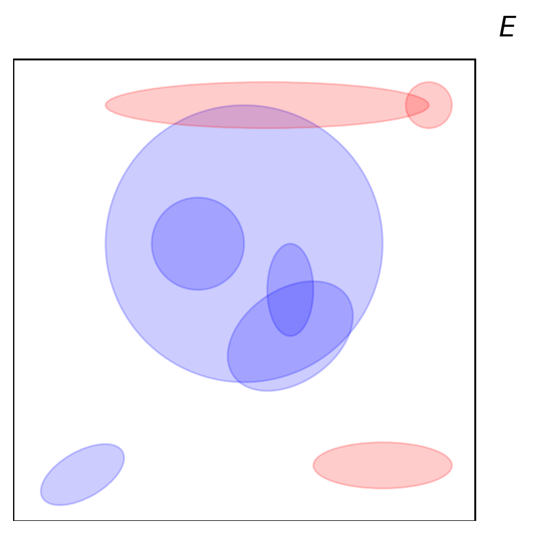
Figure 1.2: A visualisation of a universe $E$ with two collections of subsets, say $\mathcal{F}_1$ (in red, containing three elements) and $\mathcal{F}_2$ (in blue, containing five elements)

1.3 Sigma-algebras

If you think back to the Probablity Theory you know, then you’ll remember that we have some outcome (or: sample) space $\Omega$ containing all possible outcomes of our experiment, subsets of $\Omega$ are events that can either occur/happen or not, and we have a probablity measure whose job it is to assign a number from $[0,1]$ to each event (in a sensible/consistent way) representing how likely the event in question is to occur/happen if we execute the experiment once. That’s the foundations of our Probability Theory world, on which we further build beautiful buildings like random variables, stochastic processes etc. We’ll spend the rest of this chapter working towards getting that foundation established.

For starters, what subsets of $\Omega$ do we actually want to consider when we talk about “events”? The easy way forward would be to simply call any subset of $\Omega$ an event (i.e. the collection of events is then simply $\mathcal{P}(\Omega)$), because why not? Well it turns out that in general this is not always a great idea and that we need something more subtle i.e. smaller than $\mathcal{P}(\Omega)$ (which will also come in handy when we want to introduce filtrations etc. in later chapters). On the other hand, we also can’t take just any collection of subsets as our events. For instance, if $A$ and $B$ are events, then naturally we would like $A \cap B$ (“$A$ or $B$ happens”), $A \cap B$ (“$A$ and $B$ happen both”) and $A \setminus B$ (“$A$ happens but $B$ doesn’t”) also to be events no?

The natural structure to use here turns out to be a $\sigma$-algebra, also sometimes called $\sigma$-field. For the rest of this chapter we’ll use $E$ again (rather than $\Omega$) as the symbol for our universe (as we did in previous sections as well), just because this material has a much wider application than just in Probability Theory.

Definition 1.1 Consider some universe $E$ with powerset $\mathcal{P}(E)$. A collection of subsets of $E$, $\mathcal{F} \subseteq \mathcal{P}(E)$, is called a $\sigma$-algebra (on $E$) if it satisfies the following conditions:

$\emptyset \in \mathcal{F}$,
if $A \in \mathcal{F}$ then also $A^c \in \mathcal{F}$,
if $A_1, A_2, \ldots \in \mathcal{F}$ then also \[\bigcup_{i=1}^\infty A_i \in \mathcal{F}.\]

Conditions ii and iii are commonly put in words as, respectively, “$\mathcal{F}$ is closed under complements” and “$\mathcal{F}$ is closed under countable unions”.

We call a pair $(E,\mathcal{F})$ of a universe and a $\sigma$-algebra a measurable space.

Finally, observe that condition iii has consequences for any finite sequence $A_1, \ldots, A_n \in \mathcal{F}$ as well. Indeed using condition i we can extend it to an infinite sequence in $\mathcal{F}$ by setting $A_{n+1}=A_{n+2}=\ldots=\emptyset$, and as you can readily check, for condition iii to be satisfied it must hold that \[\bigcup_{i=1}^n A_i \in \mathcal{F}.\]

Here are some (prominent) examples of $\sigma$-algebras:

Example 1.3 On any universe $E$, the following collections of subsets $\mathcal{F}$ are all $\sigma$-algebras:

$\mathcal{F}=\mathcal{P}(E)$ (the powerset itself is also a $\sigma$-algebra and it is clearly the largest possible one),
$\mathcal{F}=\big\{ \emptyset, E \big\}$ (the smallest possible one),
for any subset $B \subseteq E$ fixed, $\mathcal{F}=\big\{ \emptyset, B, B^c, E \big\}$.

The conditions set out in Definition 1.1 are appropriately “minimal”⁵, we get (almost) for free that a $\sigma$-algebra is also closed under countable unions and set differences:

⁵ As you generally want in maths: you want the conditions that define some concept $X$ as “minimal” as possible (to make proving “blahblah is an $X$” as straightforward as it can be), while on the other hand you want to derive the “maximal” number of properties $X$ has i.e. the more the better, as that helps you understand the concept and is useful in later proofs to make steps like “since blahblah is an $X$, it follows that …”

Proposition 1.1 Let $\mathcal{F}$ be a $\sigma$-algebra on a universe $E$. Then:

if $A_1, A_2, \ldots \in \mathcal{F}$ then also \[\bigcap_{i=1}^\infty A_i \in \mathcal{F}\] (this also holds for finitely many elements),
if $A,B \in \mathcal{F}$ then also $A \setminus B \in \mathcal{F}$.

Proof. Ad i. We know from Definition 1.1 that a $\sigma$-algebra is closed under complements as well as (countable) unions, and now we need to deal with an intersection. A key tool to “translate” between unions and intersections are the De Morgan’s laws as discussed in Remark 1.1 ii, which allows us to write for the given $A_1, A_2, \ldots \in \mathcal{F}$ \[\left( \bigcap_{i=1}^\infty A_i \right)^c = \bigcup_{i=1}^\infty A_i^c \quad \implies \quad \bigcap_{i=1}^\infty A_i = \left( \bigcup_{i=1}^\infty A_i^c \right)^c. \tag{1.3}\] Looking at the right hand side and working “inside out”, we know that each $A_i^c \in \mathcal{F}$ (by Definition 1.1 ii), hence also the union of the $A_i^c$’s is in $\mathcal{F}$ (by Definition 1.1 iii), and hence also the complement of that union is in $\mathcal{F}$ (by again Definition 1.1 ii). So the right hand side of Equation 1.3 is in $\mathcal{F}$ and hence also the left hand side.

Ad ii. We know from Definition 1.1 and property i that a $\sigma$-algebra is closed under complements as well as (countable) unions and intersections. So our best shot is to try and rewrite a set difference in terms of these operations so that we can use these properties. Now, for the given $A,B \in \mathcal{F}$, by definition of set difference (as discussed in Section 1.2.2) we have that \[\omega \in A \setminus B \iff \omega \in A \text{ and } \omega \not\in B \iff \omega \in A \text{ and } \omega \in B^c \iff \omega \in A \cap B^c\] i.e. $A \setminus B=A \cap B^c$. Since $B \in \mathcal{F}$, also $B^c \in \mathcal{F}$ (by Definition 1.1 ii), and then it follows that also $A \cap B^c \in \mathcal{F}$ (by property i).

Finally in this section, though $\sigma$-algebras are the natural structures to work with for our purposes, they also have some challenges. A key one is that they are not so easy to specify from their basic definition. Currently the only way we have is just to list all its elements (as we did in Example Example 1.3 e.g.). That’s fine if it’s only a few of them, but for the really interesting ones that we will encounter that is not feasible. So most of the time at least we will specify the $\sigma$-algebra we want to be using in different way. Key for this is the following observation (which you should be able to convince yourself about if you think about it): the intersection of any collection of $\sigma$-algebras is itself again a $\sigma$-algebra.

This means that for any collection $\mathcal{C}$ of subsets from $E$, there exists a smallest $\sigma$-algebra $\mathcal{F}$ containing all elements of $\mathcal{C}$ i.e. so that $\mathcal{C} \subseteq \mathcal{F}$. Indeed, just take the intersection of all $\sigma$-algebras $\mathcal{F}$ satisfying $\mathcal{C} \subseteq \mathcal{F}$. We know that there is at least one such $\sigma$-algebra namely $\mathcal{P}(E)$ (cf. Example 1.3), so the result will always be a $\sigma$-algebra, either $\mathcal{P}(E)$ or a smaller one.

This observation allows us to proceed as follows: specify all the subsets of $E$ that you are particularly interested in, and then work with the smallest $\sigma$-algebra containing these subsets.

Definition 1.2 Let $\mathcal{C}$ be any collection of subsets from a universe $E$. Then there exists a smallest $\sigma$-algebra containing all elements of $\mathcal{C}$. We call this the $\sigma$-algebra generated by $\mathcal{C}$ and denote it by $\sigma(\mathcal{C})$. By “smallest” we mean that if $\mathcal{G}$ is some other $\sigma$-algebra containing all elements of $\mathcal{C}$, then $\sigma(\mathcal{C}) \subseteq \mathcal{G}$.

In addition to the basic examples listed in Example 1.3, the $\sigma$-algebras with finitely many elements are relatively easy to understand and have a very nice structure, as we’ll discuss in the next example. They are quite important as going forward we’ll often use them for inspiration/intuition!

Example 1.4 Let $E$ be any universe.

Let $A_1, \ldots, A_n$ be a partition (cf. Section 1.2.3) of $E$. Let $\mathcal{F}$ be the collection of subsets of $E$ consisting of the empty set, plus the $A_i$’s, plus any set that can be written as the union of two or more of the $A_i$’s i.e. in slightly clumsy maths \[A_{i_1} \cup A_{i_2} \cup \ldots \cup A_{i_k}, \quad \text{for some $k \in \{1,\ldots,n\}$ and $i_1, \ldots, i_k \in \{1,\ldots,n\}$.} \tag{1.4}\] Then this collection is a $\sigma$-algebra. Indeed you can easily verify the conditions in Definition 1.1 (where the partition property is crucial): the complement of a union of the form Equation 1.4 is just such a union again, made up of the “other” $A_i$’s, and the union of multiple sets of the form Equation 1.4 is (of course) again of the form Equation 1.4 — this is one of these things that is actually harder to write down than it is difficult to understand!

Note that $\mathcal{F}$ is also generated by $A_1, \ldots, A_n$ in the sense of Definition 1.2 i.e. $\mathcal{F}=\sigma(\{A_1, \ldots, A_n\})$.

Further note that $\mathcal{F}$ is finite i.e. has finitely many elements, and that (ignoring the empty set) these $A_1, \ldots, A_n$ are the “smallest” elements of $\mathcal{F}$, the building blocks which from all other elements in $\mathcal{F}$ are constructed by taking unions. We call these $A_1, \ldots, A_n$ the atoms of $\mathcal{F}$.

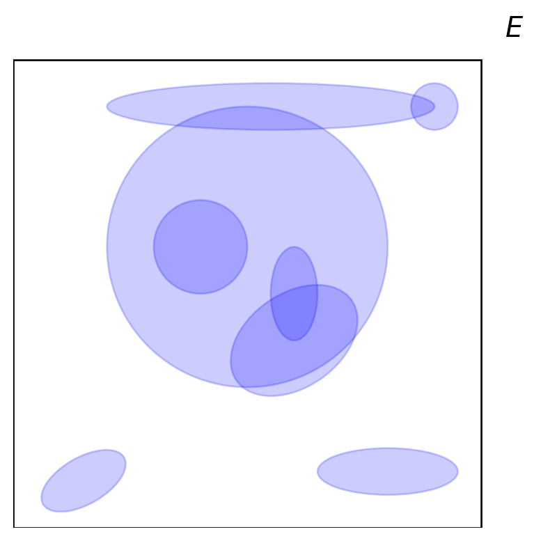
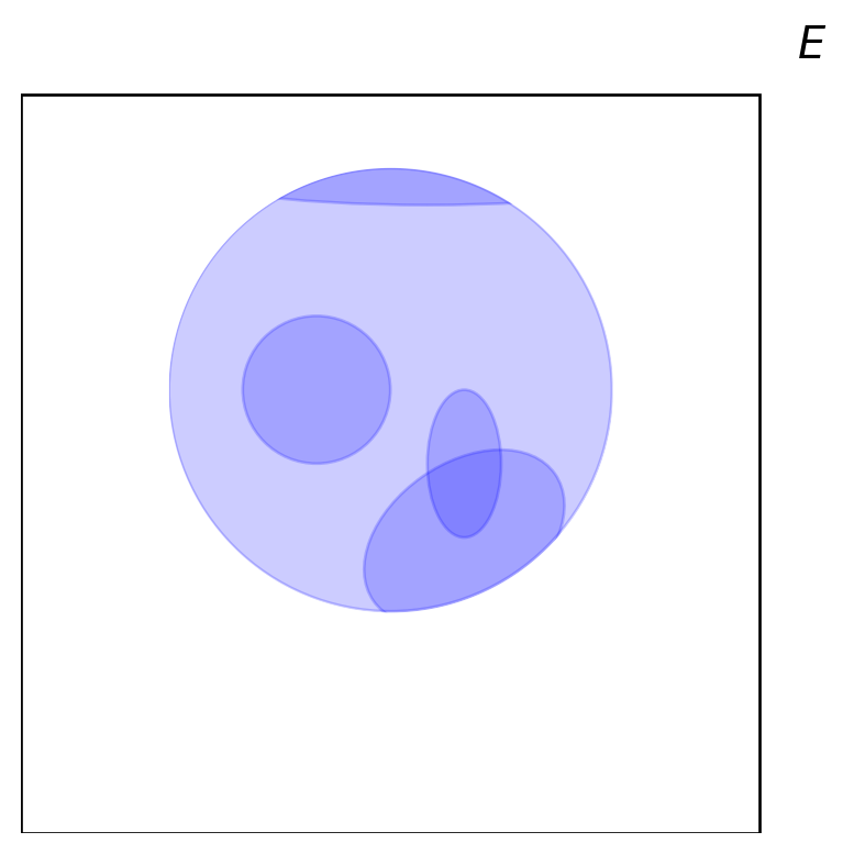
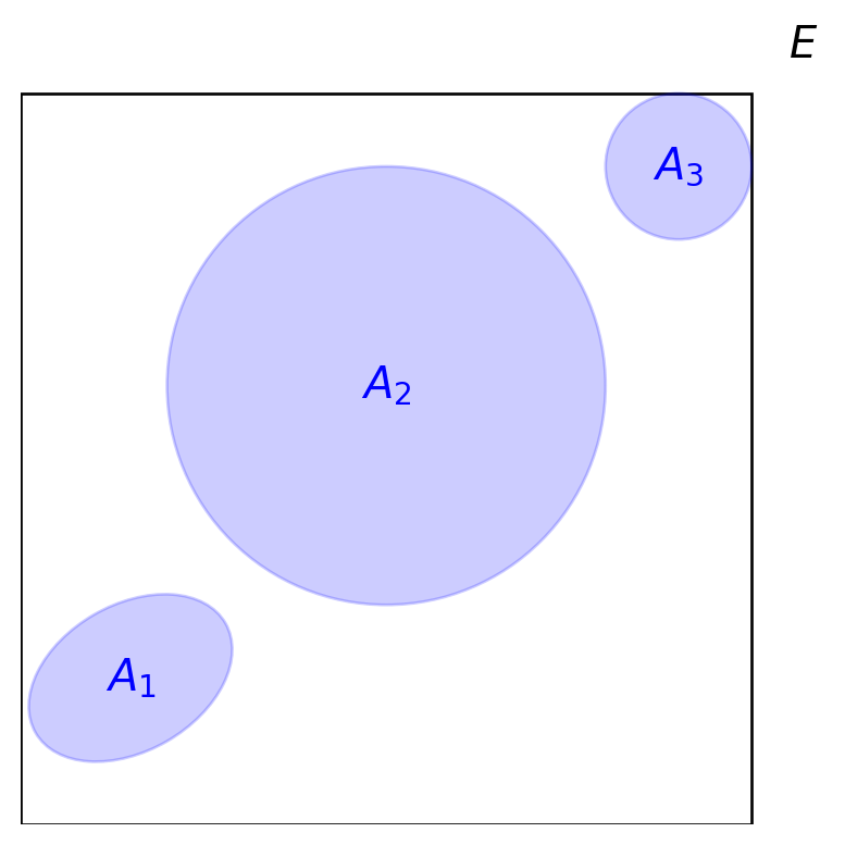
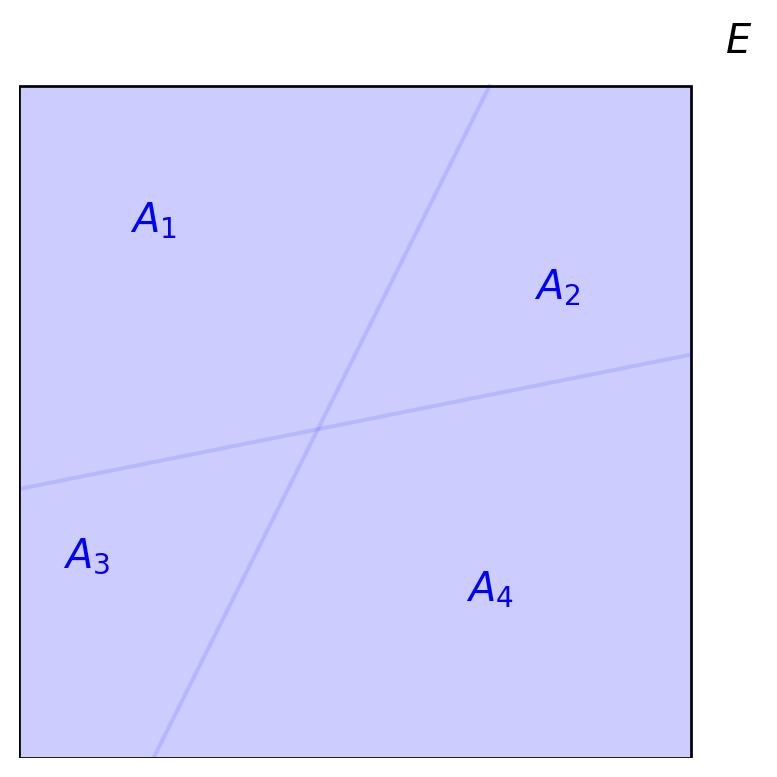
If you find the structure of $\mathcal{F}$ not so easy to see then just visualise it (poor pun intended). Take for example the situation in Figure 1.1 (b), where $A_1, \ldots, A_4$ form a partition of $\Omega$. In this case $\mathcal{F}$ consists of the empty set, the four partition elements $A_1, \ldots, A_4$ and any set that is a union of two or more of $A_1, \ldots, A_4$, e.g. $A_1 \cup A_3$, $A_2 \cup A_3 \cup A_4$ etc. etc.
The converse is also true: if $\mathcal{F}$ is any finite $\sigma$-algebra on $E$, then there exists a partition $A_1, \ldots, A_n$ of $E$ (for some $n \geq 1$) so that $\mathcal{F}$ is of the form described in the previous bullet point, with these $A_1, \ldots, A_n$ as its atoms.

For example, the $\sigma$-algebra $\big\{ \emptyset, B, B^c, E \big\}$ is of that form with $n=2$ and $A_1=B, A_2=B^c$ (check for yourself!). And, somewhat trivially, the $\sigma$-algebra $\big\{ \emptyset, E \big\}$ is also of this form with $n=1$ and $A_1=E$.

This category of $\sigma$-algebras is very nice and appealing due to their relatively simple structure. Though it’s generally a good idea to attack a problem involving $\sigma$-algebras by first assuming a finite $\sigma$-algebra with such a nice structure, keep in mind that infinite ones can generally not be understood in this form (in particular not uncountable ones) — we’ll see an example of this in Section 1.4.

Finally, note that if $E$ is itself finite then there are only finite many possible subsets of $E$ (i.e. the powerset $\mathcal{P}(E)$ is finite) and hence any $\sigma$-algebra on $E$ is necessarily finite and so of this appealing form.

Exercises

You can now do Exercise 1.1 – Exercise 1.6.

1.4 The Borel sigma-algebra

The examples of $\sigma$-algebras we encountered in the previous section are somewhat limited as they are all finite, and in particular on uncountable universes $E$ these are generally not the most interesting/useful ones. We also already mentioned that the general strategy for constructing (more complicated) $\sigma$-algebras is to generate them from a collection of subsets of special interest (cf. Definition 1.2).

It won’t surprise you that a particular universe we are interested in is the good old real line i.e. $E=\R$. Standard we like to use on this universe the $\sigma$-algebra generated by (recall Definition 1.2) all open subsets⁶ in $\R$, we call this the Borel $\sigma$-algebra⁷ on $\R$ and denote it by $\mathcal{B}(\R)$. We call any $A \in \mathcal{B}(\R)$ also a Borel (measurable) set.

⁶ Recall that a subset $A \subseteq \R$ is open if for any $x \in A$ there exists an $\eps>0$ so that $(x-\eps,x+\eps) \subseteq A$, while a subset is closed if its complement is open

⁷ All that we need to be able to define and use the Borel $\sigma$-algebra is that our universe $E$ has a proper notion of what open subsets are, which is the case for all toplogical spaces including but far from limited to $\R^n$ for $n \geq 1$ e.g.

It turns out that $\mathcal{B}(\R)$ is pretty massive! Since it contains all open subsets it also contains all closed subsets (cf. Definition 1.1 ii) and then also any finite/countable union or intersection of open/closed subsets (cf. Definition 1.1 iii and Proposition 1.1 i) etc. Of course this also applies to open/closed intervals, as our maybe most commonly used subsets of $\R$. In fact any interval $I$ is an element of $\mathcal{B}(\R)$ (see Exercise 1.7) and hence also any finite/countable union or intersection of intervals.

Since for any $x \in \R$, the set $(-\infty,x) \cup (x,\infty)$ is open and therefore an element of $\mathcal{B}(\R)$, also its complement the singleton $\{x\}$ is an element of $\mathcal{B}(\R)$. And so any finite or countably infinite subset of $\R$, i.e. any subset that we can express as $\{x_1,x_2,\ldots,x_n\}$ or $\{x_1,x_2,\ldots\}$, is also an element of $\mathcal{B}(\R)$ (as it is the finite resp. countable union of the singletons $\{x_1\}, \{x_2\}, \ldots,\{x_n\}$ resp. $\{x_1\}, \{x_2\}, \ldots$), including our famous friends $\N$, $\Z$ and $\Q$.

In fact, indeed you have to work quite hard to find/construct a subset of $\R$ that is not in $\mathcal{B}(\R)$ — in order to do so you need to dig quite deep into the fundamentals of set theory, see e.g. Vitali sets if you’re interested.

Sometimes we don’t want to consider the whole of $\R$ as our universe but rather some suitable subset, for instance an interval $I \subseteq \R$. Then we can define the Borel $\sigma$-algebra $\mathcal{B}(I)$ on the universe $I$ analogue to above, i.e. as the $\sigma$-algebra generated by all open subsets of $I$. Alternatively, we could equivalently use the technique from Exercise 1.3 to “shrink” the universe $\R$ down to the universe $I$ and $\mathcal{B}(\R)$ down to $\mathcal{B}(I)$.

Remark 1.2. It’s nice to briefly compare and contrast this one with the finite $\sigma$-algebras discussed in Example 1.4. Obviously $\mathcal{B}(\R)$ is not finite, in fact it is uncountable (cf. Section 1.2.1). We mentioned above that every singleton $\{x\}$ is a Borel set, and you may be tempted for a moment to think that we can use these as “smallest” elements in the same role as in Example 1.4. However we can’t: for starters, there are uncountably many such singletons, so they don’t provide a finite (or countable) partition of the universe $\R$. Further, in general we can’t write a set in $\mathcal{B}(\R)$ (take for instance an interval) as a finite (or countable) union of singletons. So the analogy with Example 1.4 fundamentally fails, and that nice structure from Example 1.4 is simply not present!

Ok, alright, no need to shout, I get it already — but can’t we then just use like uncountable unions or something? Did you hear that weird sound just yet, as if somebody was opening a can of beans for a full English breakfast or something? Well that’s the can of worms you have just opened and if you don’t close it again very quickly these worms, though moving slowly, will ultimately hunt you down and kill you! Uncountable unions/intersections do exist as set operations in principle, but within measure theory/Probability Theory you generally want to stay far away from them as they spell trouble. You can and will see this reflected in that whenever we deal with a union/intersection of sets in our results, it will be a countable (or finite) one. Take for instance Definition 1.1 and Proposition 1.1, the notation there is “$A_1, A_2, \ldots$” meaning that the events in question can be listed and hence it is a countable collection of events.

Exercises

You can now do Exercise 1.7.

1.5 Measures

In the above sections we have discussed how we can define a $\sigma$-algebra $\mathcal{F}$ on some universe $E$ to create a measurable space $(E,\mathcal{F})$, where the case $E=\R$ with $\mathcal{F}=\mathcal{B}(\R)$ is a particularly nice and prominent example. The last element we want to throw into the mix in this chapter is a measure. Recall that in our Probability Theory context, we need a probability measure that assigns to events (suitable subsets of our universe) a number from $[0,1]$ expressing how likely it is for that event to occur if we execute the experiment once.

But such mappings appear in other contexts as well and have many more applications: for instance, if our universe is Euclidean space ($E=\R^n$ for some $n \geq 1$) we may be interested in the length/surface/volume of a subset, or if our universe is some countable set (e.g. $E=\N$) then we may be interested in how many elements a subset has⁸ etc. Generally it is about measuring “the size” of subsets, where we can give “the size” an appropriate meaning for the context/interpretation at hand.

⁸ Of course you could also ask this question in Euclidean space but there it is much less interesting because “most” subsets (of interest) there have infinitely many elements

⁹ In this course, we use the words “mapping” and “function” interchangeably

How could we set this up mathematically? Well it needs to be a mapping⁹, say $\mu$, that assigns to each suitable subset of $E$ i.e. element of $\mathcal{F}$ some non-negative number i.e. its “size”. We want to allow for infinite “sizes” as well i.e. we allow for the range of $\mu$ to be $[0,\infty]:=[0,\infty) \cup \{\infty\}$. Further there are two fundamental properties that we would naturally want any sensible understanding of “size” to have: the empty set should have “size” $0$ (there may be other sets with “size” $0$ as well — we’ll talk more about that later), and the “size” of a union of (countably many) subsets that do not overlap/share any elements should simply be the sum of their individual “sizes”.

This brings us to the following:

Definition 1.3 Consider some measurable space $(E,\mathcal{F})$ (recall from Definition 1.1). A measure on $(E,\mathcal{F})$ is a mapping $\mu: \mathcal{F} \to [0,\infty]$ satisfying:

$\mu(\emptyset)=0$,
countable additivity (or $\sigma$-additivity): if $A_1, A_2, \ldots \in \mathcal{F}$ are mutually disjoint (recall from Section 1.2.3) then \[\mu \left( \bigcup_{i=1}^\infty A_i \right) = \sum_{i=1}^\infty \mu(A_i). \tag{1.5}\]

The resulting triplet $(E,\mathcal{F},\mu)$ consisting of a universe, a $\sigma$-algebra and a measure is called a measure space.

Some notes:

If $\mu(E)<\infty$ (recall from Exercise 1.1 that necessarily $E \in \mathcal{F}$) then we call $\mu$ a finite measure and if $\mu(E)=1$ then we call $\mu$ (can you guess it??) a probability measure. (Note that it follows from Theorem 1.1 i that $\mu(E)$ is the largest value $\mu$ can take, which provides context for this comment).
Note that, analogue to the same point in Definition 1.1 really, any finite sequence $A_1, A_2, \ldots, A_n \in \mathcal{F}$ of mutually disjoint events can be extended to an infinite one by setting $A_{n+1}=A_{n+2}=\ldots=\emptyset$ and applying Equation 1.5 to this infinite sequence yields \[\mu \left( \bigcup_{i=1}^n A_i \right) = \sum_{i=1}^n \mu(A_i).\]

We’ll discuss some examples of measures (in particular on $(\R,\mathcal{B}(\R))$) in the next section, and we’ll also discuss the special case of finite/countable universes $E$ further below. However the study of measure spaces in general (as well as more specific and advanced examples) goes way beyond what we have time and scope for in this course, we are only focusing on the parts that are most useful in Probability Theory/that we will need in the course. If you are interested in a bit more then see e.g. Stroock (1994, chap. VII) and the references therein.

Here are some of the key properties that measures have — they will be ringing a few bells with you, since you’ll have seen and used most/all of them as properties of a probability measure in your earlier Probability courses! We will leave the proofs up to you in the exercises.

Theorem 1.1 Let $(E,\mathcal{F},\mu)$ be a measure space. Then the following holds.

For the first two properties, let $A, B \in \mathcal{F}$.

Suppose that $A \subseteq B$. Then $\mu(A) \leq \mu(B)$. If $\mu(A)<\infty$, then also $\mu(B \setminus A)=\mu(B)-\mu(A)$.
If $\mu(A \cap B)<\infty$ then $\mu(A \cup B)=\mu(A)+\mu(B)-\mu(A \cap B)$.

For the remaining properties, let $A_1, A_2, \ldots \in \mathcal{F}$.

Subadditivity: it holds that (compare and contrast with Equation 1.5) \[\mu \left( \bigcup_{i=1}^\infty A_i \right) \leq \sum_{i=1}^\infty \mu(A_i) \tag{1.6}\] (note that the obvious analogue holds for a finite sequence $A_1,\ldots,A_n$ as well — just set $A_{n+1}=A_{n+2}=\ldots=\emptyset$ and apply Equation 1.6).
If $A_1, A_2, \ldots$ is a non-decreasing sequence i.e. $A_1 \subseteq A_2 \subseteq \ldots$ then it has a limit $A$ (in $\mathcal{F}$, cf. Definition 1.1 iii) which we can e.g. express as \[A = \bigcup_{i=1}^\infty A_i\] and we have that \[\mu(A)=\lim_{i \to \infty} \mu(A_i).\]
Similarly, if $A_1, A_2, \ldots$ is a non-increasing sequence i.e. $A_1 \supseteq A_2 \supseteq \ldots$ then it has a limit $A$ (in $\mathcal{F}$, cf. Proposition 1.1 i) which we can e.g. express as \[A = \bigcap_{i=1}^\infty A_i\] and provided that $\mu(A_1)<\infty$ we again have that \[\mu(A)=\lim_{i \to \infty} \mu(A_i).\]

Some notes:

Properties iv and v express a notion of “continuity” of a measure: if sets $A_i$ tend to some limit set $A$ (in a monotone fashion), then $\mu(A_i)$ tends to $\mu(A)$.
Properties i, ii and v contain a finiteness condition which is trivially satisfied if $\mu$ is a finite measure or probability measure.

We conclude with a discussion of countable vs uncountable universes $E$ (recall from Section 1.2.1):

Remark 1.3. Recall that, as mentioned in Section 1.1, ultimately the motivation for the work we are doing in this chapter is to build a framework for our Probability Theory that can handle any random experiment we throw at it by generalising notions we intuitively understand for random experiments with only finitely many possible outcomes. We do this by putting no restriction on our universe $E$ (which will later, when we narrow our focus from measure theory to Probability Theory, play the role of our outcome/sample space $\Omega$): it can can have finitely many elements but also countably infinite or even uncountably many elements.

As we’ll learn, and indeed can see now a bit as well, as long as we stay within the realm of a countably infinite universe $E$ then our intuition for experiments with only finitely many elements extends pretty naturally. We could call these “simple” experiments. However if we cross that faultline and venture into the world of uncountable universes things get a bit more spicy! We could call these “advanced” experiments.

Forget (for a moment only please :() everything we have discussed so far. Let’s go back to the experiment of rolling a die. How do we compute probabilities there? Well we have an outcome space containing only six elements, say $\Omega=\{1,2,3,4,5,6\}$, and well, we know that each possible outcome has probability $1/6$ and we can compute any probability we need from there no? True! But hang on, so we didn’t need to specify a $\sigma$-algebra of subsets that are our “events” at all, and aren’t we supposed to use Definition 1.3 to define a (probability) measure as a mapping that assigns a probablity from $[0,1]$ to each event?? Well, yes and no. ;).

The framework that we have introduced so far is necessary to cover “advanced” experiments (the above approach generally won’t work anymore) but it is general and also covers “simple” experiments. It’s just that you don’t really (need to) see things in terms of that general framework when you do only “simple” experiments, and so you typically don’t get to see it (at least not in a lot of detail) in your basic Probability courses.

To illustrate the connection between our general framework on the one hand and our more direct intuiton for “simple” cases on the other hand, let’s go back from the Probability focus to the slightly more general meausre spaces context again, i.e. rather than $\Omega$ we use $E$ and rather than a probability measure we use a measure $\mu$. Take a finite or countable universe, say $E=\{\omega_1,\omega_2,\ldots,\omega_n\}$ or $E=\{\omega_1,\omega_2,\ldots\}$. Then we could have proceeded as follows. Trivially, any $A \subseteq E$ can be written as a finite or countable union of its elements as singletons i.e. (bit awkward to express in a formula) \[A = \bigcup_{\omega_i \in A} \{\omega_i\}. \tag{1.7}\] Any mapping $\mu$ on subsets of $E$ (with values in $[0,\infty]$) with the countable additivity property (recall from Definition 1.3) then satisfies \[\mu(A)=\sum_i \mu(\{\omega_i\}). \tag{1.8}\] This equation tells us the following: if we know the value that $\mu$ assigns to all the singletons $\{\omega_i\}$, then we also know/can compute the measure of any $A \subseteq E$. No need for a $\sigma$-algebra (well, the $\sigma$-algebra is simply the powerset $\mathcal{P}(E)$), and any possible measure (incl. probability measure obviously) is fully determined by the value it assigns to the singletons. And that is, of course, exactly how our intuition for “simple” experiments like the rolling a die above works: we assign probabilities to each of the possible outcomes, and any other probablity that we are interested in naturally follows, by making use of Equation 1.8. (In the case of rolling a die, we have $E=\{\omega_1,\ldots,\omega_6\}$ and $\mu(\{\omega_i\})=1/6$, so that for any event/subset $A \subseteq E$ we get that $\mu(A)=|A|/6$, where $|A|$ denotes the number of elements in $A$.)

Contrast this with the case of an uncountable $E$, like $E=\R$ for instance (the “advanced” case). Interesting subsets of $\R$, like an interval, contain uncountably many elements (i.e. real numbers) and hence cannot be written as a countable union of singletons (as also already observed in Remark 1.2) i.e. Equation 1.7 is no longer possible. That means that also the whole construction of (probability) measures by simply assigning values to singletons no longer works, for one reason because we can’t use Equation 1.8 any longer to extend it to larger sets. That is the key reason why in general, we must define measures as mappings acting on subsets rather than just on singletons/elements in $E$.

Another complication is that in the uncountable case, it is generally (surprisingly!) not possible to define a (non-trivial) measure on all subsets i.e. there simply does not exist a (non-trivial) mapping satisfying the conditions in Definition 1.3 and with as domain the powerset $\mathcal{P}(E)$ (we’ll see an example of this in Section 1.6.1). That’s the reason that we were forced to introduce $\sigma$-algebras (although they’ll come in handy later in the context of martingales in a different light as well), so that we can still define and work with measures, albeit we have to accept on a smaller domain than $\mathcal{P}(E)$.

(These are some of the dragons we promised at the end of Section 1.2.1!)

Exercises

You can now do Exercise 1.8 – Exercise 1.11.

1.6 Measures on the Borel sigma-algebra

In Section 1.4 we discussed the Borel $\sigma$-algebra on $\R$ to create the measurable space $(\R,\mathcal{B}(\R))$, and already mentioned that it is a particularly interesting case (for us). Now we have defined what measures are in Section 1.5, it only makes sense to wrap up this chapter with a brief discussion of measures on this measurable space.

1.6.1 The Lebesgue measure

The (arguably) most prominent example of a measure in the context of uncountable universes in general, is the Lebesgue measure $\lambda$ on the measure space $(\R,\mathcal{B}(\R))$.

Recall from the introduction in Section 1.5 that the notion of a measure in general was motivated by wanting a mathematically rigorous understanding of the “size” of a set. What could that look like in $\R$? Well, for starters, for any interval $I$ a natural understanding of “size” would be its length (no matter whether it is open or closed at either end point). That is to say, we are looking for a measure $\lambda$ (in the sense of Definition 1.3) that satisfies for any $a<b$ \[\lambda([a,b])=\lambda((a,b])=\lambda([a,b))=\lambda((a,b))=b-a \tag{1.9}\] and also for intervals of infinite length, including $\R=(-\infty,\infty)$ itself: \[\lambda((-\infty,a])=\lambda((-\infty,a))=\lambda((a,\infty))=\lambda([a,\infty))=\lambda(\R)=\infty. \tag{1.10}\] Now the hunt is on to construct (or at least show the existence of) such a measure on the whole of $\mathcal{B}(\R)$ i.e. a mapping $\lambda: \mathcal{B}(\R) \to [0,\infty]$ satisfying the properties the conditions of Definition 1.3 (so in particular countable additivity) and satisyfing Equation 1.9 & Equation 1.10! This measure naturally extends the concept of “size”/“length” to any Borel set.

The details of this construction are beyond the scope of this course (see Stroock 1994, chap. II e.g. if you are interested), we’ll settle for saying “it can be done” (but it does require some work!). An interesting consequence of the (typical) construction is that you can actually define $\lambda$ on a larger $\sigma$-algebra than just $\mathcal{B}(\R)$ (the sets in this larger $\sigma$-algebra are called, not surprisingly, the Lebesgue measurable sets). However this $\sigma$-algebra is still smaller than the powerset $\mathcal{P}(\R)$ i.e. there do exist subsets of $\R$ that are not Lebesgue measurable¹⁰! On the other hand, for the purposes of this course you don’t need to be worry about these too much — to give you some feel: it follows from the above that any not Lebesgue measurable set is also not Borel measurable, and recall the discussion we had in Section 1.4 about how unlikely you are to run into not Borel measurable sets “in the wild”.

¹⁰ If you were to try to define the Lebesgue measure on the whole of $\mathcal{P}(\R)$, then you’ll run into trouble such as that the countable additivity property from Definition 1.3 no longer holds in general. At least, that is the case if you accept the usual axioms around set theory etc. There do exist different approaches to set theory i.e. based on different axioms that avoid such problems, but then these come with their own, ehm, peculiarities ;)

As a final point, if you don’t want to have the whole of $\R$ as your universe but rather only on some (Borel measurable) subset, say an interval $I$, then we have seen before (recall Exercise 1.3) that $(I,\mathcal{B}(I))$ is a measurable space. The Lebesgue measure also naturally lives on such a space, e.g. following the “zooming in” procedure as seen in Exercise 1.3. A particularly interesting choice for us is the universe $I=(0,1)$, since then the Lebesgue measure of the whole universe is $\lambda((0,1))=1-0=1$ i.e. the Lebesgue measure is a probability measure (recall from Definition 1.3) in this context! Further, just for interest: you can define the Lebesgue measure in similar vein on Borel sets in the universe $\R^n$ for $n \geq 2$ as well, in that case you start with replacing Equation 1.9 by the obvious analogue for rectangles (if $n=2$), cuboids (if $n=3$) or higher dimensional analogues.

Proposition 1.2 On the measure space $(\R,\mathcal{B}(\R))$ (or $(I,\mathcal{B}(I))$ for some interval $I \subseteq \R$) the Lebesgue measure $\lambda: \mathcal{B}(\R) \to [0,\infty]$ can be defined. It works on intervals according to Equation 1.9 and Equation 1.10. Further it of course satisfies all the properties from Definition 1.3 and Theorem 1.1.

Some notable facts, to get a little bit of a feel for the guy despite our only brief discussion:

Any open Borel set $A \in \mathcal{B}(\R)$ can be expressed as a countable union of mutually disjoint open intervals (see e.g. Stroock 1994, Lemma 2.1.9) and hence, by countable additivity (cf. Definition 1.3) and Equation 1.9 & Equation 1.10, $\lambda(A)$ equals the sum of the lengths of these intervals.
Any countable subset $A$ of $\R$ (which is always a Borel set, recall from Section 1.4) has Lebesgue measure $0$ i.e. $\lambda(A)=0$ (cf. Exercise 1.13). This makes some sense intuitively maybe: it is tempting to consider a countable subset as “quite small” in the context of the uncountably many real numbers. However see iv below.
This is one to chew on for a bit (at least I remember that was the case for me when I first encountered this as student): there do also exist uncountable Borel sets with Lebesgue measure $0$ (a particularly famous example is the Cantor set)!
More chewing (maybe)! Recall that the set of rational numbers $\Q$ is dense in $\R$ i.e. for any $r \in \R$ and for any $h>0$, there exists a $q \in \Q$ so that $|r-q|<h$. Indeed, write down the decimal expansion of $r$ and keep only the first $n$ digits. The result is a rational number, and you can get it arbitrarily close to $r$ by only making $n$ large enough. However, despite that denseness, $\lambda(\R)=\infty$ while $\lambda(\Q)=0$ (due to countability, see ii above)…

Remark 1.4. In Remark 1.3 we already alluded to the fact that while in “simple” situations of countable universes any measure is fully specified by how it acts on the singletons, this nice and simple construction dramatically breaks down in “advanced” cases where the universe is uncountable.

Indeed in the context of $E=\R$, by Equation 1.9 any interval $[a,b]$ has a positive Lebesgue measure $\lambda([a,b])=b-a>0$. On the other hand, any interval is “just” a collection of real numbers. Yet as Proposition 1.2 ii states, any singleton $\{x\}$ has Lebesgue measure $0$. So somehow, the Lebesgue measure of the interval (i.e. $b-a>0$) is not equal to the sum of Lebesgue measures of singletons (which would be $0$)!! What, is our celebrated countable additivity property (cf. Definition 1.3) suddenly failing us?? No it isn’t — the point is that an interval, being uncountable (cf. Section 1.2.1), is not a countable union of these singletons and hence the countable additivity property was not expected to apply in the first place!

It’s the promised dragons again — and I urged you in Remark 1.2 already to leave that can of worms that is uncountable unions(/intersections) firmly closed! You can also see iii and iv in Proposition 1.2 in the same light.

So the key message is: in an uncountable universe $E$, be extra careful with double checking that something that seems obvious is indeed actually true (by proving it from the definitions and results we have already and will later collect, and checking that you’re indeed working with finite/countable unions/intersections etc).

Exercises

You can now do Exercise 1.12–Exercise 1.14.

1.6.2 Other measures

Of course, the Lebesgue measure is far from the only one you could define on the Borel sets — after all, even though the Lebesgue measure is natural if we want to interpret “size” as length, that doesn’t mean we couldn’t use other interpretations (or indeed just put that interpretation to the side altogether)! In this section we explore other possible measures, in particular finite ones (not only for their own interest but also because they will pop up quite prominently in our Probablity Theory context later, after all a probability measure is finite).

This section is in particular for those of you interested and for occasional (technical) reference later on — do have a read through but don’t worry about the nitty gritty details for exam purposes, in particular not the proof of Lemma 1.2.

A key role in this section is played by the collection of all intervals of the form $(-\infty,x]$ for $x \in \R$, let’s call this collection $\mathcal{C}$. Let’s first observe that this collection can be used as generator (cf. Definition 1.2) for the Borel $\sigma$-algebra (cf. Section 1.4):

Lemma 1.1 Define the following collection of subsets of $\R$: \[\mathcal{C}=\{ (-\infty,x] \, | \, x \in \R \}.\] Then we have that $\sigma(\mathcal{C})=\mathcal{B}(\R)$.

Proof. Note that for any $a<b$, \[(a,b]=(-\infty,b] \setminus (-\infty,a] \in \sigma(\mathcal{C})\] (cf. Proposition 1.1 ii) and hence also \[(a,b)=\bigcup_{i=1}^\infty (a,b-1/i] \in \sigma(\mathcal{C})\] (cf. Definition 1.1 iii). Since any open set in $\R$ can be written as a countable union of open intervals (cf. Lemma 2.1.9 in Stroock (1994)), it follows from Definition 1.1 iii that any open set in $\R$ is also an element of $\sigma(\mathcal{C})$. Since $\mathcal{B}(\R)$ is generated by the open sets in $\R$, we get that $\mathcal{B}(\R) \subseteq \sigma(\mathcal{C})$.

On the other hand, since any interval of the form $(-\infty,x]$ is a Borel set (cf. Exercise 1.7) we also have that $\sigma(\mathcal{C}) \subseteq \mathcal{B}(\R)$ and hence the result follows.

Now, let’s think about other possible measures on the Borel sets $\mathcal{B}(\R)$. How would you go about investigating/constructing those? It seems like a bit of a daunting task: we have already discussed that (non-trivial) $\sigma$-algebras such as $\mathcal{B}(\R)$ are complicated beasts, not very easy to oversee/specify which subsets of $\R$ it exactly contains and which not, and in order to define a measure on it we need to specify a mapping that sends each of its elements (that we can hardly specify in the first place) to a non-negative number, while the mapping also needs to satisfy the conditions in Definition 1.3!

Hmm. We discussed previously that we can get a handle on $\sigma$-algebras (at least to some extent) by working with easier to understand collections that generate it. Like $\mathcal{B}(\R)$ is by definition generated by all open subsets in $\R$ (cf. Section 1.4), and as Lemma 1.1 shows also by the simpler collection $\mathcal{C}$ (in general, any (non-trivial) $\sigma$-algebra has many possible generators). This line of thinking naturally leads to the following idea/question: would it maybe be possible to characterise/define a measure on the whole of $\mathcal{B}(\R)$ by initially defining it on a simpler collection that generates $\mathcal{B}(\R)$ only? The answer is yes, at least, if we consider finite measures only and as long as you choose a generating collection with some particular properties. And, as you had probably guessed, $\mathcal{C}$ is exactly a collection that fits the bill here!

Here is a quick analogy to illustrate the process. Suppose that we have a box of Lego bricks in different shapes and sizes. We want to define a function that takes as input any possible building we can make with these bricks, and gives us back the weight of the building. It would be one hell of a job to sit down, put together all possible buildings you can make and weigh them (to specify our function exhaustively). Rather it would make more sense to only weigh the individual bricks and jot the results down. Then whenever we construct some building, which is a sequence of steps in which we add and sometimes take away bricks, the total weight and hence the value of my function naturally follows if at each step we keep track of the weight of the bricks that are added/removed: its value is naturally extended from/determined by the individual bricks in whatever building we fancy making.

A measure on $(\R,\mathcal{B}(\R))$ needs, by definition, to give us a value (think: weight) for any Borel set (think: any possible building we could make). However we also know that a measure should be countably additive, cf. Definition 1.3 (think: it should respect the principle that the weight of any building equals the sum of the weights of the individual bricks). So, if we can identify what the collection of bricks should be ($\mathcal{C}$ is a possible choice), then the value it assigns to any Borel set is fully characterised by the values it assigns to the elements of $\mathcal{C}$!

In Lemma 1.2 we work out this idea. It shows that any finite measure on the Borel sets is fully specified by the values it assigns to the elements of $\mathcal{C}$, and vice versa that if we choose any (suitable) values to assign to the elements of $\mathcal{C}$ then these choices extend to a finite measure on all Borel sets. In order to conveniently talk about “(suitable) values assigned to the elements of $\mathcal{C}$”, note that for every $x \in \R$ there is one corresponding element in $\mathcal{C}$ namely $(-\infty,x]$, i.e. for every $x \in \R$ we need one value, so we may well represent these values as a function $f: \R \to [0,\infty)$, where $f(x)$ is the value we assign to $(-\infty,x]$ for all $x \in \R$.

Finally a word about the “suitable” in the above “(suitable) values assigned to the elements of $\mathcal{C}$”: a finite measure takes values in $[0,\infty)$ and hence so should $f$. Further as $x$ increases, the interval $(-\infty,x]$ gets larger, hence keeping in mind Theorem 1.1 i we should have that $f$ is non-decreasing. Further as we let $x \to -\infty$ the interval $(-\infty,x]$ collapses to the empty set and hence, by Theorem 1.1 v and Definition 1.3, we should have that $f(x) \to 0$. If we let $x \to \infty$ then $(-\infty,x]$ grows to become $\R$ and hence by Theorem 1.1 iv we should have that $f(x)$ tends to some finite limit which is the measure of $\R$.

Lemma 1.2 Denote by $\mathbf{F}$ the family of all functions $f: \R \to [0,\infty)$ that are right-continuous, non-decreasing and satisfy \[\lim_{x \to -\infty} f(x)=0 \quad \text{and} \quad \lim_{x \to \infty} f(x)<\infty\] (note that both limits are guaranteed to exist since $f$ is non-decreasing), and by $\mathbf{M}$ the family of all finite measures on $(\R,\mathcal{B}(\R))$.

Then the mapping that sends $\mu \in \mathbf{M}$ to the function $f: \R \to [0,\infty)$ given by $f(x):=\mu((-\infty,x])$ is a bijection (i.e. creates a one-to-one correspondence) between $\mathbf{M}$ and $\mathbf{F}$. That is, each $\mu \in \mathbf{M}$ is mapped to a unique $f \in \mathbf{F}$ (injective) and for every $f \in \mathbf{F}$ a $\mu \in \mathbf{M}$ exists that gets mapped to it (surjective).

Some notes:

Recall that a function is right-continuous on $\R$ if for every $x \in \R$, $f(x+h) \to f(x)$ as $h \downarrow 0$. Of course, this does not necessarily mean that $f$ is also continuous in $x$, after all the left hand limit $\lim_{h \downarrow 0} f(x-h)$ may not exist or not be equal to $f(x)$. However if such a function is also non-decreasing then it cannot get too wild, for instance it must be continuous everywhere on $\R$ except for in at most countably many points (see e.g. Wiki).
This result remains true if we work on an interval $I=(a,b)$ e.g. rather than the whole of $\R$, in the way that you would expect: take for $\mathbf{M}$ all finite measures on $(I,\mathcal{B}(I))$, for $\mathbf{F}$ all right-continuous, non-decreasing functions $f: I \to [0,\infty)$ with limit value $0$ resp. finite if $x \downarrow 0$ and $x \uparrow b$ resp., and map $\mu \in \mathbf{M}$ to $f$ given by $f(x):=\mu((a,x])$.
Following up on the previous bullet point, since on an interval $I=(a,b)$ the Lebesgue measure is finite (cf. Section 1.6.1), it should be covered by this lemma as well. Indeed what function does it get mapped to??
The function $f$ associated with a $\mu \in \mathbf{M}$ is called its distribution function. Though we’re in measure theory mode here rather than in Probability Theory mode, you may very well already see the parallels with our use of (almost) that word in Probability Theory — we’ll return to this later on!

Proof. Let $\mathcal{C}$ be as defined in Lemma 1.1. First we need to show that for a $\mu \in \mathbf{M}$, the function $f: \R \to [0,\infty)$ given by $f(x):=\mu((-\infty,x])$ is indeed a member of $\mathbf{F}$ i.e. satisfies the conditions set out in the lemma. We’ll leave this as an exercise for later.

Injective. If $\mu, \nu \in \mathbf{M}$ get mapped to the same function then they coincide on all elements of $\mathcal{C}$. But then necessarily $\mu=\nu$. This is due to the fact that $\mathcal{C}$ is closed under finite intersections (i.e. it is a so-called $\pi$-system), see e.g. Lemma 3.1.3 and Exercise 3.1.8 in Stroock (1994).

Surjective. The difficulty here is to show that, roughly speaking, if you specify values that you would would like your measure to have for elements in $\mathcal{C}$, that a measure on the whole of $\mathcal{B}(\R)$ actually exists respecting these values. We can’t go from $\mathcal{C}$ to the whole of $\mathcal{B}(\R)$ directly but need to use another collection of subsets as intermediate step.

Consider the collection $\mathcal{A}$ of all subsets $A \subseteq \R$ that can be written as \[A=I_1 \cup I_2 \cup \ldots \cup I_n \quad \text{for some $n \geq 1$}, \tag{1.11}\] where each $I_i$ takes one of the following forms:

$(-\infty,a]$ for some $a \in \R$,
$(a,b]$ for some $a,b \in \R$ with $a<b$,
or $(b,\infty)$ for some $b \in \R \cup \{-\infty\}$.

We also include $\emptyset$ in $\mathcal{A}$ (the case $n=0$ if you will). Note that for any pair of such intervals that are not disjoint, their union can be simplified to a single interval of one of these three forms, so we can assume without loss of generality that the $I_i$’s used in Equation 1.11 are disjoint.

This collection has the special property that it is closed under complements as well as finite unions (for the latter, just convince yourself that the union of two elements from $\mathcal{A}$ is again in $\mathcal{A}$) i.e. it is a so-called algebra.

Note that $\mathcal{C} \subseteq \mathcal{A}$ and hence $\sigma(\mathcal{C}) \subseteq \sigma(\mathcal{A})$. Using Lemma 1.1 we get that $\mathcal{B}(\R) \subseteq \sigma(\mathcal{A})$. On the other hand, any interval is a Borel set (cf. Exercise 1.7), hence so is any element of $\mathcal{A}$ (cf. Definition 1.1 iii), and therefore $\sigma(\mathcal{A}) \subseteq \mathcal{B}(\R)$. Altogether: $\sigma(\mathcal{A})=\mathcal{B}(\R)$.

Given some $f \in \mathbf{F}$, define the mapping $\mu: \mathcal{A} \to [0,\infty)$ by first setting \[\begin{aligned} & \mu(\emptyset)=0, \quad \mu((-\infty,a])=f(a), \\ & \mu((a,b])=f(b)-f(a) \quad \text{and} \quad \mu((b,\infty))=f(\infty)-f(b), \end{aligned} \] where $f(\infty):=\lim_{x \to \infty} f(x)$ (note that all of these are non-negative since $f$ is non-decreasing), and then for any $A=I_1 \cup I_2 \cup \ldots \cup I_n \in \mathcal{A}$ (where, recall, we assume that the $I_j$’s are disjoint) we set \[\mu(A)=\sum_{j=1}^n \mu(I_j). \tag{1.12}\]

We need to prove two properties of $\mu$ before we can make the final step. The first property is finite additivity (i.e. as in Definition 1.1 but for only finitely many disjoint elements of $\mathcal{A}$). For this it is enough to show that for disjoint $A_1, A_2 \in \mathcal{A}$ we have that \[\mu(A_1 \cup A_2)=\mu(A_1)+\mu(A_2), \tag{1.13}\] then finite additivity follows by mathematical induction e.g. However this is pretty obvious: if two sets of the form Equation 1.11 are disjoint, then all the intervals used to express them must be mutually disjoint, so that Equation 1.13 follows immediately from Equation 1.12 (of course, this argument can also be used to show finite additivity directly, but the possibility to use mathematical induction here as well is nice to observe as a useful tool in other similar situations).

The second property we need to show is that if $A_1 \supseteq A_2 \supseteq ... \in \mathcal{A}$ is a “decreasing” sequence of sets that tend to the empty set i.e. \[\bigcap_{i=1}^\infty A_i = \emptyset, \tag{1.14}\] then $\mu(A_i) \to 0$ as $i \to \infty$. For this, first assume that in the expression Equation 1.11 $A_1$ contains only intervals of the form $I_j=(a,b]$. Then in $A_2 \subseteq A_1$, each $I_j$ is either no longer present or it has become another interval of the same form, contained in $I_j$. This observation can be repeated in $A_3 \subseteq A_2$ etc.: we can follow each of the original $I_j$’s in $A_1$ separately through their own “shrinking process” as we let $i$ increase and walk through the $A_i$’s. Due to Equation 1.12, the claim follows if we can show that each $I_j$ ultimately “shrinks” to a limit set with $0$ measure.

So fix any of these $I_j$’s in $A_1$ and write it as $(a_1,b_1]$. If it vanishes i.e. becomes the empty set at any step in the process then its measure becomes $0$ at that step and there is nothing more to do. Assume now that this doesn’t happen i.e. that for each $i=2,3,\ldots$, $A_i$ contains $(a_i,b_i]$ with $a_i<b_i$, $a_i \geq a_{i-1}$ and $b_i \leq b_{i-1}$. Since the $a_i$’s and $b_i$’s each form a monotone sequence they each have a limit, say $a_\infty$ and $b_\infty$. Since $a_i<b_i$ for all $i \geq 1$, $a_\infty \leq b_\infty$. It can’t be true that $a_\infty < b_\infty$ because then the non-empty interval $(a_\infty,b_\infty]$ is a subset of each $A_i$ and hence of the intersection of all $A_i$’s, violating Equation 1.14. So we know that $a_\infty = b_\infty$. Further it also can’t happen that $a_i<a_\infty=b_\infty$ for all $i \geq 1$, because then the singleton $\{a_\infty\}$ is a subset of each $A_i$, again violating Equation 1.14.

Now, we get from the def of $\mu$ that \[\mu((a_i,b_i])=f(b_i)-f(a_i)=f(b_i)-f(b_\infty)+f(a_\infty)-f(a_i).\] We have to be slightly careful here because $f$ is not necessarily continuous (in the point $a_\infty = b_\infty$) but we do know that it is right-continuous. Hence $f(b_i)-f(b_\infty) \to 0$ as $i \to \infty$. Further as we’ve seen above, for all $i$ large enough we have $a_i=a_\infty$ and hence $f(a_\infty)-f(a_i)=0$. In conclusion, indeed $\mu((a_i,b_i]) \to 0$ as $i \to \infty$. And, reiterating the earlier observation, by our assumption that $A_1$ consists only of intervals of the form $(a,b]$ and by Equation 1.12, $\mu(A_i) \to 0$ as $i \to \infty$.

Ok – getting there! It remains to consider the cases where $A_1$ also contains an interval of the form $(-\infty,a_1]$ and/or $(b_1,\infty)$. In the former case, as we walk through the $A_i$’s in the “shrinking process”, one of the following things happen: the interval $(-\infty,a_1]$ vanishes (in which case there is nothing to show), or at some point in the process it becomes one or more intervals of the form $(c,d]$ for $c>-\infty$ and $d \leq a_1$ in which case we can apply the above arguments again, or otherwise each of the $A_i$’s contains an interval of the form $(-\infty,a_i]$ with $a_i \leq a_{i+1}$ and limit say $a_\infty$. In this latter situation, in order to satisfy Equation 1.14 it must be true that $a_\infty=-\infty$, and we can derive our desired conclusion that its measure vanishes from the property $\lim_{x \to -\infty} f(x)=0$. In an analogue manner you can deal with an interval of the form $(b_1,\infty)$.

Right! Now we finally have everything in place to be able to apply the majestic Caratheodory Extension Theorem (see e.g. Corollary 7.1.22 in Stroock (1994)), which guarantees that a finite measure $\mu$ exists on $\sigma(\mathcal{A})=\mathcal{B}(\R)$ which respects/is an extension of the mapping $\mu$ we defined on $\mathcal{A}$, and hence in particular it also has the property that $\mu((-\infty,x])=f(x)$ for all $x \in \R$.

As a final note: the Caratheodory Extension Theorem in fact guarantees uniqueness of the measure as well, but it is worthwhile to see the $\pi$-system argument we used to show the injectivity property as that is a much more direct and commonly used argument in similar situations.

In a way this lemma may be a bit sobering: it implies that measures can effectively be reduced to a family of relatively easy to understand, good old functions. Is that really all there is, is there nothing more exciting? There sure is! Crucially important is that this lemma addresses finite measures only. The ones that are not finite are not (all) so easily captured!

1.7 Some exercises

About the exercises

Each exercise has a (rough) indication of its difficulty, as follows:

*	easier: can be solved by (almost) only using relevant definitions/results,
**	medium: in addition to relevant definitions/results, needs a limited amount of work/creativity,
*******	harder: in addition to relevant definitions/results, needs a larger amount of work/serious creativity,
💀	warning: might make your brain hurt! These are mainly intended to provide some extra challenge for those of you keen on that and are generally quite hard. You don't need to worry about these too much for exam purposes.

The exam consists of mostly ** and *** level questions, some *, and possibly at most a few marks worth of 💀.

A bit of preaching: it is an incredibly important part of the study process to try and work on the exercises as much as possible. To become a better mathematician/learn new maths (and also to get a good exam mark ;)), above all you need to do it. And yes, of course that includes falling over things, and making mistakes, and getting stuck, and getting frustrated — all part of the game and what you’re supposed to be doing! Your lecturers have done that as well and still do it. What matters is that you don’t let that discourage you and that you make good use of the help and resources available to help you develop your skills. As part of that, many exercises have a hint in a block like this:

Hint (click to view)

Hint!

These are trying to help you on your way if you don’t know where to start or to provide some ideas if you get stuck. In spirit of the above, always have a look at these first and try again before you look at the full solution. (These hints are an extra service that won’t be available in the exam I’m afraid ;).)

Of course, we have our classes and there’s office hours, email etc. as well — I’m at any time very happy to help you with any questions you may have, and you should please never feel that any question is “too dumb” to ask!

Full/detailed solutions for the exercises will become available, just immediately below the exercises, after our Friday tutorial.

Exercise 1.1 [*] Let $E$ be any universe and $\mathcal{F}$ a $\sigma$-algebra on $E$. Prove that $E \in \mathcal{F}$.

Full solution (click to view)

From Definition 1.1 i we have that $\emptyset \in \mathcal{F}$, and it follows from Definition 1.1 ii that also $\emptyset^c=E \in \mathcal{F}$.

Exercise 1.2 [*] Consider a universe consisting of five elements, say $E=\{x_1,\ldots,x_5\}$. Consider the following collection of subsets of $E$: $\mathcal{F}=\big\{ \emptyset, \{x_2,x_3\},\{x_1,x_4,x_5\},E\big\}$. Is $\mathcal{F}$ a $\sigma$-algebra?

Hint: one-liner using the examples we have seen!

Full solution (click to view)

This is just the third example in Example 1.3 with $B=\{x_2,x_3\}$, so indeed a $\sigma$-algebra!

Exercise 1.3 [**/***] Let $\mathcal{F}$ be a $\sigma$-algebra on some universe $E$. Fix some $B \in \mathcal{F}$. Let $\mathcal{G}=\{ A \cap B \, | \, A \in \mathcal{F} \}$, i.e. the collection of all subsets of $E$ that are of the form $A \cap B$ for some $A \in \mathcal{F}$. Prove that $\mathcal{G}$ is a $\sigma$-algebra on the universe $B$.

Some notes:

What happens here is that you effectively ‘zoom in’ from your original universe $E$ to the smaller subset $B$ as your new universe. You create $\mathcal{G}$ on $B$ by going through all elements $A$ in $\mathcal{F}$ and only keeping the part of $A$ that lies in $B$ (if any). The result is a collections of subsets that are all contained in your new universe $B$, and as this exercise shows it even conveniently inherits the $\sigma$-algebra properties from $\mathcal{F}$! This construction is visually illustrated in Figure 1.3.
It is important to appreciate that we consider $\mathcal{G}$ in the context of the universe $B$. For instance, in this context the complement of a set $A \in \mathcal{G}$ is the set $\{ \omega \in B \, | \, \omega \not\in A\}$ (compare with the expression for complement in Section 1.2.2 e.g.).

Full solution (click to view)

We need to check that the collection $\mathcal{G}$ satisfies all three conditions from Definition 1.1, which we can do as follows:

Since $\mathcal{F}$ is a $\sigma$-algebra, we know that $\emptyset \in \mathcal{F}$ (by Definition 1.1 i). Hence by def of $\mathcal{G}$, $\emptyset \cap B \in \mathcal{G}$. Of course $\emptyset \cap B=\emptyset$ so indeed $\emptyset \in \mathcal{G}$.
Pick any $A \in \mathcal{G}$. This means that we can write $A=C \cap B$ for some $C \in \mathcal{F}$, and (hence) in particular $A \subseteq B$. Now note that the complement of $A$ in the universe $B$ (recall the second bullet point above) can e.g. be expressed as \[\{ \omega \in B \, | \, \omega \not\in A\}=B \cap A^c=B \cap (C \cap B)^c.\] In order to show that this guy is in $\mathcal{G}$, by def of $\mathcal{G}$ we need to show that $(C \cap B)^c \in \mathcal{F}$. But we know that $B$ and $C$ are both in $\mathcal{F}$, hence so is their intersection (by Proposition 1.1 i) and hence also the complement of that intersection (by Definition 1.1 i).
Finally, let $A_1, A_2, \ldots \in \mathcal{G}$, which by def of $\mathcal{G}$ means that there are $C_1, C_2, \ldots \in \mathcal{F}$ so that $A_i=C_i \cap B$ for all $i \geq 1$. Now we can e.g. write \[\bigcup_{i=1}^\infty A_i = \bigcup_{i=1}^\infty (C_i \cap B) = \left( \bigcup_{i=1}^\infty C_i \right) \cap B\] (the final step by the distributivity property). So in order to show that this union of $A_i$’s is in $\mathcal{G}$, by def of $\mathcal{G}$ we need to show that the union of the $C_i$’s is in $\mathcal{F}$. But this holds since $C_1, C_2, \ldots \in \mathcal{F}$ and by Definition 1.1 iii.

Exercise 1.4 [*] In some (non-empty) universe $E$, let $B \subset E$ with $B \not= \emptyset$. Set $\mathcal{C}=\{B\}$. What is the $\sigma$-algebra generated by $\mathcal{C}$ i.e. $\sigma(\mathcal{C})$? What is $\sigma(\mathcal{C})$ if $B=\emptyset$? And what if $B=E$?

Hint (click to view)

All answers are $\sigma$-algebras that we have already encountered!

Full solution (click to view)

Recall from Definition 1.2 that $\sigma(\mathcal{C})$ is the smallest $\sigma$-algebra containing all the elements (i.e. subsets of $E$) that are present in $\mathcal{C}$. In this case it is hence the smallest $\sigma$-algebra that contains $B$ as one of it elements. Now, if the $\sigma$-algebra contains $B$ then it must also contain $B^c$ (to satisfy Definition 1.1 ii). Further it must contain $\emptyset$ (to satisfy Definition 1.1 i) and also its complement i.e. $E$ (again to satisfy Definition 1.1 ii). So, so far we have that $\sigma(\mathcal{C})$ should contain at least $\emptyset$, $B$, $B^c$ and $E$. But this is also enough, since we know already that this collection indeed forms a $\sigma$-algebra (cf. Example 1.3 and Exercise 1.2). We should also convince ourselves that it is the smallest $\sigma$-algebra, but the previous arguments already show that each of the four elements must really be present. In conclusion: $\sigma(\mathcal{C})=\{ \emptyset, B, B^c, E\}$.

When $B=\emptyset$ i.e. $\mathcal{C}=\{\emptyset\}$, by the same arguments as above, the $\sigma$-algebra should at least contain $\emptyset$ itself as well as its complement $E$. Anything else? Well no, because the collection consisting of these two elements already makes a $\sigma$-algebra (cf. Example 1.3 and Exercise 1.2). So we can conclude that $\sigma(\mathcal{C})=\{ \emptyset, E\}$.

Finally, when $B=E$ we get by the same arguments as in the previous paragraph that again $\sigma(\mathcal{C})=\{ \emptyset, E\}$.

Exercise 1.5 [*] Let $\mathcal{F}$ be a $\sigma$-algebra on some universe $E$. What is $\sigma(\mathcal{F})$?

Full solution (click to view)

Recall again from Definition 1.2 that for any collection of subsets $\mathcal{C}$, $\sigma(\mathcal{C})$ is the smallest $\sigma$-algebra containing all the elements that are present in $\mathcal{C}$. Well, but $\mathcal{F}$ itself is a $\sigma$-algebra which trivially contains every element also present in $\mathcal{F}$ no? And clearly there is no smaller $\sigma$-algebra that also contains all the elements of $\mathcal{F}$ than $\mathcal{F}$ itself? So indeed: $\sigma(\mathcal{F})=\mathcal{F}$.

Exercise 1.6 [*/**] Let $E$ be a finite universe. We mentioned before already that its powerset, $\mathcal{P}(E)$, is (trivially) a $\sigma$-algebra and it’s also (trivially) finite. In Example 1.4 we discussed that any finite $\sigma$-algebra contains atoms $A_1, \ldots, A_n \subseteq E$ from which all elements (other than $\emptyset$) in the $\sigma$-algebra can be constructed by taking unions. What are the atoms in the case of $\mathcal{P}(E)$?

Full solution (click to view)

The atoms of $\mathcal{P}(E)$ are simply all elements of the finite $E$ as singletons, i.e. if we write $E=\{x_1,\ldots,x_n\}$ then the atoms are $A_1=\{x_1\}$, $A_2=\{x_2\}$, …, $A_n=\{x_n\}$. Indeed any element of $\mathcal{P}(E)$ i.e. any subset of $E$ can (trivially) be written as the union of its elements as singletons. So the $\sigma$-algebra generated by these atoms is the whole of $\mathcal{P}(E)$. On the other hand, any other partition of $E$ contains a subset with at least two elements, say $x_i$ and $x_j$. The $\sigma$-algebra generated by that partition (i.e. by means of taking unions) does not contain $\{x_i\}$ and $\{x_j\}$. So this $\sigma$-algebra does not contain all subsets of $E$ and is hence not $\mathcal{P}(E)$.

Exercise 1.7 [*/**] Let $a,b \in \R$ with $a<b$. We know from Section 1.4 that all open and all closed subsets of $\R$ are elements of $\mathcal{B}(\R)$. Show that the intervals $(a,b]$ and $[a,b)$ are also elements of $\mathcal{B}(\R)$.

Hint (click to view)

What are their complements? Are these in $\mathcal{B}(\R)$?

Full solution (click to view)

Note that each interval is neither open nor closed. For $I=(a,b]$, we have that $I^c=(-\infty,a] \cup (b,\infty)$. Now $(-\infty,a]$ is closed and hence in $\mathcal{B}(\R)$, $(b,\infty)$ is open and hence also in $\mathcal{B}(\R)$. So also their union i.e. $I^c$ is in $\mathcal{B}(\R)$ (cf. Definition 1.1 iii). Since $I$ is the complement of its complement i.e. $I=(I^c)^c$ also $I$ is in $\mathcal{B}(\R)$.

The analogue works for $I=[a,b)$.

Note: this is far from the only possible proof, any valid proof is fine of course.

Exercise 1.8 [*/**] Consider some universe $E$ with $\sigma$-algebra $\mathcal{F}$, and let $\mu: \mathcal{F} \to [0,\infty]$ be a mapping satisyfing the countable additivity condition of Definition 1.3. Suppose that an $A \in \mathcal{F}$ exists with $\mu(A)<\infty$. Show that it follows that $\mu(\emptyset)=0$.

Note: this shows that any mapping $\mu: \mathcal{F} \to [0,\infty]$ satisyfing countable additivity is either a measure, or it trivially maps each $A \in \mathcal{F}$ to $\infty$.

Full solution (click to view)

If you’re not sure where to start with something like this, just write down the few things that you do know/are given and play a bit around with them. In this case, all we really have is an $A \in \mathcal{F}$ with $\mu(A)<\infty$, and we know that $\mu$ satisfies countable additivity. We want to try and say something about $\mu(\emptyset)$. Ok, what happens if we apply the countable additivity to the two (indeed disjoint) sets $A$ and $\emptyset$? Well it gives us that \[\mu(A \cup \emptyset) = \mu(A)+\mu(\emptyset).\] Of course $A \cup \emptyset=A$ so the left hand side is just $\mu(A)$, and it indeed follows that $\mu(\emptyset)=\mu(A)-\mu(A)=0$.

Note that how this argument would fail if $\mu(A)=\infty$, since then we’d get $\mu(\emptyset)=\infty-\infty$ which is an undefined quantity.

Exercise 1.9 [*/**] Briefly explain, e.g. via an example, why in Equation 1.6 we only have an inequality while in Equation 1.5 we have an equality.

Full solution (click to view)

In Equation 1.6 we do not make the assumption that the sets are mutually disjoint i.e. we allow the sets to overlap. Then when we add up the measures of the sets we “double count” (or triple, or …) the measures of intersections between sets. As an extreme example, fix some set $A \in \mathcal{F}$ and set $A_1=A_2=\ldots=A_n:=A$. Then on the one hand \[\mu \left( \bigcup_{i=1}^\infty A_i \right)=\mu(A)\] while on the other hand \[\sum_{i=1}^n \mu(A_i) = \sum_{i=1}^n \mu(A)=n \mu(A)\] so clearly they are far from equal.

Exercise 1.10 [*/**] On the measurable space $(\R,\mathcal{B}(\R))$, in each of the below cases find out what the limit of the sequence of sets is (in the sense of Theorem 1.1 iv and v), provided it exists.

$A_k=(-k,k)$ for $k=1,2,\ldots$
$A_k=(1-1/k,1+1/k)$ for $k=1,2,\ldots$
$A_k=[1-1/k,1+1/k]$ for $k=1,2,\ldots$.

Hint (click to view)

Recall that in Remark 1.1 iv we discuss how to interpret/define infinite unions and intersections.

Full solution (click to view)

This is an increasing sequence of intervals and so the limit exists (and equals the union of all $A_k$’s). Intuitively it is clear that this sequence will ultimately fill up the whole of our universe $\R$. Indeed, take any $x \in \R$. Then $x \in A_k$ for all $k$ large enough (larger than $|x|$ e.g.) and hence also $x \in \cup_{k=1}^\infty A_k$. So indeed $\cup_{k=1}^\infty A_k=\R$.
This is a decreasing sequence of intervals and so the limit exists (and equals the intersection of all $A_k$’s). Intuitively, as $k$ grows $A_k$ is an ever shorter interval around $1$ and hence we would guess that the limit is the singleton $\{1\}$. To make this rigorous, note that each $A_k$ contains $1$ and hence also $1 \in \cap_{k=1}^\infty A_k$. For any $x \not= 1$, for $k$ large enough we have that $x \not\in A_k$ (e.g. when $1/k<|x-1|$ i.e. $k>1/|x-1|$) and hence also $x \not\in \cap_{k=1}^\infty A_k$. In conclusion, indeed $\cap_{k=1}^\infty A_k=\{1\}$.
Same argument and end answer as in ii!

Exercise 1.11 [**/***] Prove properties i–iv of Theorem 1.1 (you can do v as well if you like, but it is quite similar to iv).

Maybe you want to leave property iii to do last — that’s probably the trickiest one!

Hint (click to view)

Recall that from its definition, Definition 1.3, we only know how to compute the measure of the empty set and of a finite or countable union of mutually disjoint sets. So if we want to derive an expression for the measure of anything else, we’ll need to try and express that “anything else” in terms of the empty set/a finite or countable union of mutually disjoint sets. Recall also that Venn diagrams can be quite handy!

Full solution (click to view)

Note: all sets we create in these solutions consist of unions/intersections/differences of sets that we assume to be in $\mathcal{F}$ (as part of the assumptions in Theorem 1.1), hence from Definition 1.1 & Proposition 1.1 we know that all these created sets are also in $\mathcal{F}$ and that hence they are valid arguments for the measure $\mu$.

We do properties i and ii first:

Since $A \subseteq B$, we can write $B$ as the union of two disjoint sets as follows: $B=A \cup (B \setminus A)$ (use Venn diagram e.g.). From Definition 1.3 ii it follows that $\mu(B)=\mu(A)+\mu(B \setminus A)$. Since $\mu(B \setminus A) \geq 0$, we indeed get that $\mu(B) \geq \mu(A)$. We also get that $\mu(B \setminus A)=\mu(B)-\mu(A)$ provided that $\mu(A)<\infty$ (otherwise we would end up with the undefined $\infty-\infty$ in the right hand side).
Looking to write $A \cup B$ as the union of mutually disjoint sets, we can e.g. do that as $A \cup B=A \cup (B \setminus (A \cap B))$ (use Venn diagram e.g.). So, provided that $\mu(A \cap B)<\infty$: \[\mu(A \cup B)=\mu(A \cup (B \setminus (A \cap B)))=\mu(A)+\mu(B \setminus (A \cap B)) =\mu(A)+\mu(B)-\mu(A \cap B),\] where the second equality uses Definition 1.3 ii and the third uses the result of part i above (indeed $A \cap B \subseteq B$).

Next we do property iv. Recall from Definition 1.3 that essentially the only real tool we have for dealing with a sequence of subsets $A_1, A_2, \ldots$ is countable additivity, but this requires the subsets to be mutually disjoint which is clearly not the case for the non-decreasing sequence of events we’re dealing with here. So we need to figure out a way to bring mutually disjoint sets into play! The key observation is that we may write for any $n \geq 1$ \[\begin{align*} A_n &= A_1 \cup A_2 \setminus A_1 \cup A_3 \setminus A_2 \cup \ldots \cup A_n \setminus A_{n-1} \\ &= \bigcup_{j=1}^n B_j, \end{align*} \tag{1.15}\] where we define $B_1:=A_1$, $B_j := A_j \setminus A_{j-1}$ for all $j \geq 2$. If you don’t see what’s going on here, draw a pic of a growing sequence of sets $A_1$, $A_2$, $A_3$ and see where these set differences fit into your pic. The beauty of this is that the sequence $B_1, B_2, \ldots$ is mutually disjoint, and hence by countable additivity (cf. Definition 1.3 ii) it follows that for any $n \geq 1$ \[\mu(A_n)=\sum_{j=1}^n \mu(B_j). \tag{1.16}\] Further we claim that we may write the limit set $A$ as the union of the $B_j$’s: \[A=\bigcup_{j=1}^\infty B_j. \tag{1.17}\] To see that this holds, first pick any element $\omega \in A$. By def of $A$, i.e. $A=\cup_{n=1}^\infty A_n$, there must exist an $n$ so that $\omega \in A_n$. By Equation 1.15, also $\omega \in \cup_{j=1}^n B_j$ and hence also $\omega \in \cup_{j=1}^\infty B_j$. The other way around, pick any element $\omega \in \cup_{j=1}^\infty B_j$. Then there must exist an $i$ so that $\omega \in B_i$. Again by Equation 1.15, it follows that $\omega \in A_n$ for all $n \geq i$ and hence also $\omega \in \cup_{n=1}^\infty A_n$.

Finally, having established Equation 1.17, since the $B_j$’s are mutually disjoint, we can apply countable additivity to get \[\mu(A)=\mu \left( \bigcup_{j=1}^\infty B_j \right) = \sum_{j=1}^\infty \mu(B_j)\] and using that an infinite sum is nothing but the limit of partial sums and Equation 1.16 we get exactly what we were looking for: \[\mu(A)=\lim_{n \to \infty} \sum_{j=1}^n \mu(B_j) = \lim_{n \to \infty} \mu(A_n).\] Done!

Finally it remains to do property iii. This is one of these where the thing you want to prove seems fairly obvious (after all it translates to: the “size” of a union can never be larger than the sum of the “sizes” of the components) but then it is not so clear how to actually go about it. There is a few ways to do it (and any valid way is fine of course). One way is to do something similar as we did in the proof of property iv. Another route is to observe that property ii above implies a simplified version of the claim: $\mu(A \cup B) \leq \mu(A)+\mu(B)$. Maybe we can throw some mathematical induction add this to extend it beyond two sets?

Ok, for starters, note that we can safely assume that $\mu(A_i)<\infty$ for all $i \geq 1$. After all, if that were not true then $\sum_{i=1}^\infty \mu(A_i)=\infty$ and the statement we are trying to prove is trivially true. Next let’s use induction to prove that for any $n \geq 2$ it holds that \[\mu \left( \bigcup_{i=1}^n A_i \right) \leq \sum_{i=1}^n \mu(A_i). \tag{1.18}\] For this, the “base case” with $n=2$ follows from property ii. For the “induction step”, take any $n \geq 3$ and assume that Equation 1.18 holds for $n-1$ (the “induction hypothesis”). Then we can deduce \[\mu \left( \bigcup_{i=1}^n A_i \right) = \mu \left( A_n \cup \bigcup_{i=1}^{n-1} A_i \right) \leq \mu(A_n) + \mu \left( \bigcup_{i=1}^{n-1} A_i \right) \leq \mu(A_n) + \sum_{i=1}^{n-1} \mu(A_i) = \sum_{i=1}^{n} \mu(A_i),\] where the first inequality uses property ii (applied to the sets $A_n$ and $\cup_{i=1}^{n-1} A_i$) and the second the “induction hypothesis”. So we have now completed the induction process and proven that Equation 1.18 indeed holds for all $n \geq 2$.

Be aware that this is still not entirely what we need to prove though. The obvious way to try and extend this to the statement we need is to take the limit for $n \to \infty$ at both sides of Equation 1.18. That gives us what we want on the right hand side, but not really on the left hand side: we get a limit in front of the $\mu$ while we actually need it inside the $\mu$. Note that you can’t just put the limit inside without any further ado because this is not always valid/true, it needs a proof that you can do that! It essentially needs a “continuity” property of $\mu$, of which we have seen two specific formulations in properties iv and v. So let’s see if we can use those. We could for instance define $B_n := \cup_{i=1}^n A_i$ for all $n \geq 1$. Then the $B_n$’s form a non-decreasing sequence (if we increase $n$ we only add more sets to the union so it definitely doesn’t get any smaller) and you can easily check that (*): \[\bigcup_{n=1}^\infty B_n = \bigcup_{i=1}^\infty A_i.\] Using this we then finally arrive at our result: \[\mu \left( \bigcup_{i=1}^\infty A_i \right) =\mu \left( \bigcup_{n=1}^\infty B_n \right) = \lim_{n \to \infty} \mu(B_n) = \lim_{n \to \infty} \mu \left( \bigcup_{i=1}^n A_i \right) \leq \lim_{n \to \infty} \sum_{i=1}^n \mu(A_i) = \sum_{i=1}^\infty \mu(A_i),\] where the second equality uses property iv, the third the definition of $B_n$, and the inequality uses Equation 1.18. Done!

(*): if you’re not entirely sure how to do this: recall Remark 1.1 iii (and iv). To show that the union of $B_n$’s is a subset of the union of the $A_i$’s, if $x$ is an element of the union of the $B_n$’s then it must be an element of $B_n$ for some $n$. By def of $B_n$ it is then also an element of $\cup_{i=1}^n A_i$, and so it must be an element of one of $A_1, \ldots, A_n$. But then it also an element of the union of all $A_i$’s. You can go the other way by yourself!

Exercise 1.12 [*] For each of the following three (Borel measurable) sets, compute its Lebesgue measure.

$A=[5,10)$,
$A=[1,2] \cup (3,4)$,
the set $A$ consisting of all intervals of the form $(k,k+r^k)$ for all $k=1,2,\ldots$, for some $r \in (0,1)$.

Full solution (click to view)

Directly from Equation 1.9 we get that $\lambda([5,10))=10-5=5$.
Since $A$ is given as the union of two disjoint intervals, by countable addivitivy (cf. Definition 1.3) and Equation 1.9 we can compute $\lambda([1,2] \cup (3,4))=\lambda([1,2])+\lambda(3,4))=2-1+4-3=2$.
Note that can write \[A=\bigcup_{k=1}^\infty (k,k+r^k)\] and since $r^k \leq 1$ for all $k=1,2,\ldots$, this is a union of mutually disjoint intervals. Again by countable addivitivy (cf. Definition 1.3) and Equation 1.9 we find \[\lambda \left( \bigcup_{k=1}^\infty (k,k+r^k) \right) = \sum_{k=1}^\infty \lambda((k,k+r^k)) = \sum_{k=1}^\infty k+r^k-k = \sum_{k=1}^\infty r^k = \frac{r}{1-r},\] the final step by the good old geometric series.

Exercise 1.13 [**] Prove that on the measure space $(\R,\mathcal{B}(\R),\lambda)$, where $\lambda$ is the Lebesgue measure, any countable $A \in \mathcal{B}(\R)$ has Lebesgue measure $0$ i.e. $\lambda(A)=0$.

Hint (click to view)

First show that the Lebesgue measure of a singleton equals $0$. For this you only need Equation 1.9!

Full solution (click to view)

First consider a singleton $\{x\}$ for any $x \in \R$, we’d like to show that it has Lebesgue measure $0$. A simple way to do that is to pick any $y>x$ and write $[x,y]=\{x\} \cup (x,y]$, so that by countable additivity (cf. Definition 1.3) and Equation 1.9 we can deduce \[\lambda([x,y])=\lambda(\{x\})+\lambda((x,y]) \implies \lambda(\{x\})=\lambda((x,y])-\lambda([x,y])=y-x-(y-x)=0.\] Now, any countable set can be written as a list of elements (recall from Section 1.2.1) i.e. either in the form $\{x_1,\ldots,x_n\}$ or $\{x_1,x_2,\ldots\}$. Since such a set can be expressed as a union of singletons (in each singleton one of its elements), by countable additivity the Lebesgue measure of the set is the sum of the Lebesgue measures of these singletons, which by the above indeed boils down to $0$.

(Note that all the sets we use in this answer are guaranteed to be Borel measurable, cf. Section 1.4, so we know that they have a well defined Lebesgue measure)

Exercise 1.14 [**] Show that in fact, Equation 1.10 follows from Equation 1.9. That is to say, assume that you know that the Lebesgue measure $\lambda$ satisfies Equation 1.9, now prove that Equation 1.10 follows. How many different proofs can you come up with??

Full solution (click to view)

Take the case $I=[a,\infty)$ for some $a \in \R$. Here are some proofs I could think of.

We could for instance use Theorem 1.1 i: for any $n \geq 1$ we have that $[a,a+n) \subseteq I$ and hence by Theorem 1.1 i and Equation 1.9 $\lambda(I) \geq \lambda([a,a+n))=a+n-a=n$. It follows that $\lambda(I)=\infty$ (otherwise, if $\lambda(I)<\infty$ we would get a contradiction for all $n$ large enough).
We could also use countable additivity (cf. Definition 1.3) yet again: write $I$ as a union of mutually disjoint intervals, e.g. $[a,a+1), [a+1,a+2), \ldots$ so that by countable additivity and Equation 1.9 it follows that \[\begin{aligned} \lambda(I) &= \lambda \left( \bigcup_{n=1}^\infty [a+n,a+n+1) \right) \\ &= \sum_{n=1}^\infty \lambda([a+n,a+n+1)) \\ &=\sum_{n=1}^\infty a+n+1-(a+n) \\ &= \sum_{n=1}^\infty 1 = \infty. \end{aligned} \]
But we could also use a limit: take e.g. $I_n := [a,a+n)$ for $n \geq 1$. This forms an increasing sequence of sets with as limit $I$ in the sense of Theorem 1.1 iv: \[I=\bigcup_{n=1}^\infty I_n\] and it follows from Theorem 1.1 iv and Equation 1.9 that \[\lambda(I)=\lim_{n \to \infty} \lambda(I_n)=\lim_{n \to \infty} a+n-a = \lim_{n \to \infty} n=\infty.\]

(a) Some universe $E$ with a collection of subsets (the purple shapes, some of which overlap i.e. have non-empty intersection) $\mathcal{F}$ (note that this collection is **not** a $\sigma$-algebra, just to avoid getting a visual with too many subsets — doesn’t affect the construction principle though!)