5 Stochastic processes & martingales (in discrete time)

5.1 Why?

Well just because we now finally can! After four chapters of preparing the grounds and building the foundations, we are now ready to march on and start looking at stochastic processes and in particular martingales. The coming chapters are devoted to stochastic processes/martingales in discrete time.

Obviously we will still rely on and use in particular the key results from the previous chapters. In particular conditional expectations are central to the definition and hence applications of martingales — we’ll use the results from Section 4.6 a lot!

Martingales form one of the most important classes of stochastic processes (not even an “arguably” this time!) with many applications — financial mathematics is one of these but also many others, including in fields like engineering, biology, economics etc. but also within maths: in statistics, parts of applied and pure maths, as well as, more close to home, as fundamental building blocks within the vast field of stochastic processes and applications.

As we introduce and discuss first examples and properties of martingales in this chapter, you’ll see a very famous name pop up a few times, that of Joseph Doob, an American mathematician who is truly a founding father of this material. It is maybe nice to point out that Doob did his work from about the 1940s onwwards, and he died only in 2004. This comes on the back of the development of modern Probability Theory, as discussed in the previous chapters, for which the Russian mathematician Andrey Kolmogorov was a pivotal force in the 1930s in particular. All this just to say the following. Much of the maths that you get to see as undergraduate student is quite old — parts famously going back as far as the ancient Greeks and beyond. In that light, all of this stuff is very new and recent mathematics — though I appreciate that it will feel less recent to you than it does to me!

5.2 The basics of a stochastic process (in discrete time)

In essence a stochastic process (in discrete time) is nothing but a (countable) sequence of random variables on some probablity space $(\Omega,\mathcal{F},\P)$, say $X_0, X_1, \ldots$, as we have already briefly looked at in Section 2.6 and Section 2.7 for instance. Sometimes we’ll also look at the case of a finite collection $X_0, X_1, \ldots, X_N$ for some $N \in \N$ but we’ll take in principle the point of view of an infinite sequence. We’ll typically write the collection as $(X_n)_{n=0,1,\ldots}$ (or $(X_n)_{n=0,1,\ldots,N}$ in the finite case).

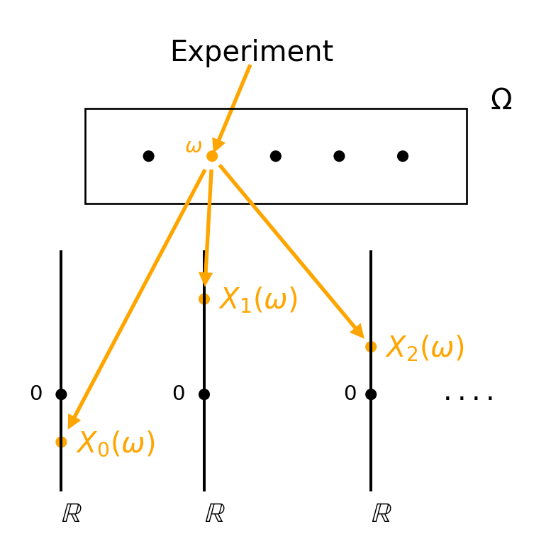
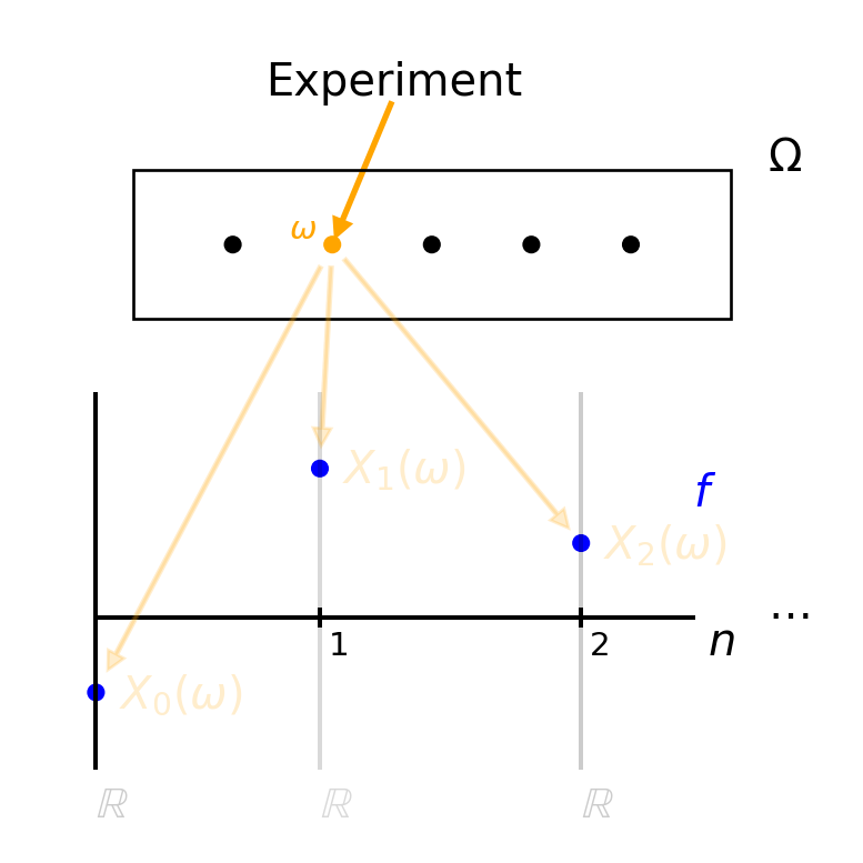
The basic mental model is the same as in previous chapters: an experiment is executed yielding an outcome $\omega \in \Omega$ (with $\P$ describing the likelihoods of events i.e. $\mathcal{F}$-measurable subsets $A \subseteq \Omega$ happening) and then each random variable takes a value, yielding a sequence $X_0(\omega), X_1(\omega), \ldots$ of real numbers that we tend to call a path or realisation (some people use also, as in the single random variable case, simply the word sample). Although it is of course “just” a sequence of real numbers, we have a favourite way of visualising/looking at such a path/realisation: as (the plot of) a function from $\N$ to $\R$, given by $n \mapsto X_n(\omega)$ for $n \in \N$. See also Figure 5.1.

(a) Starting from the visualisation in Figure 2.3 for two random variables, we now extend that to an infinite sequence $X_0, X_1, \ldots$ (and we display the real lines vertically). Note that all the structure from Figure 2.3 is still present here as well: you can choose Borel sets on any/all of the real lines, consider their inverse images etc.

Then we add a little bit of sauce to our (mental) model to make it more interesting. Crucially for our discussion of martingales as a particular class of stochastic processes (as well as many other classes of stochastic processes), we think about the index $n$ as time (in whatever unit), i.e. we imagine that the horizontal axis in Figure 5.1 (b) represents a time axis (with often $n=0$ as “now”) and that as time progresses, the values $X_0(\omega), X_1(\omega), \ldots$ are gradually revealed to us. Typically $X_0$ will be a trivial constant random variable (reflecting the fact that $n=0$ is “now” and hence we already know its value), mostly $X_0=0$. Note that this interpretation doesn’t contradict with the fact that once the experiment is done and $\omega \in \Omega$ chosen, all values $X_0(\omega), X_1(\omega), \ldots$ are fixed, we just imagine that they get revealed to us in order, one every minute say.

It is important to realise that in (interesting examples of) stochastic processes, the random variables are not independent¹ — independent sequences are a bit boring. That comes with the consequence that as time goes on and more values get revealed to us, the amount of information available to us increases and we (generally) gain “prediction power” of the values of the random variables that haven’t yet been revealed to us.

¹ Indeed, you could argue that studying stochastic processes is all about studying dependency structures between random variables

Example 5.1 Here is a quick example: imagine that a die is rolled infinitely often and that $X_n$ denotes the average of the first $n$ rolls (with $X_0:=0$ say). Even though the results of the individual rolls are independent, the $X_n$’s are clearly not: $X_n$ and $X_{n+1}$ both use the result of the first $n$ rolls. In fact, as a quick computation shows, with $Y_{n+1}$ the result of the $(n+1)$-th dice roll, we can write \[X_{n+1}=\frac{1}{n+1} Y_{n+1}+\frac{n}{n+1} X_n\] which shows that as $n$ grows, the influence of the “unpredictable” element $Y_{n+1}$ on the value of $X_{n+1}$ decreases while (hence) the influence of $X_n$ grows. So, indeed: the larger $n$ gets, the more “prediction power” for $X_{n+1}$ we gain if we know $X_n$. Obviously this is a particularly nice and simple example, in general these structures may be much more hidden and harder to see/quantify.

We mentioned above “amount of information” and “prediction power”. But hang on, we have tools to make such things more precise: $\sigma$-algebras to represent amounts/levels of information (cf. Remark 4.3) and for “prediction” we have conditional expectations, both from the previous Chapter 4! Hold that thought for a moment, in order to write it down we first need to look at a few more aspects of $\sigma$-algebras that are useful in this context.

Recall that in Definition 2.2 we introduced the notion of the $\sigma$-algebra generated by a function/random variable: it is the smallest $\sigma$-algebra that makes the function/random variable in question measurable (cf. Definition 2.1) and it is easy to write down: it’s just the collection of all inverse images of the Borel sets (it should contain at least these sets to make the function/random variable measurable, but conveniently these sets do make up a $\sigma$-algebra so we don’t need to make the collection any larger to get the $\sigma$-algebra properties so to speak). Here is a quick and helpful result that extends this idea to multiple functions/random variables (for a proof, see e.g. Section 3.13 in Williams (1991)):

Lemma 5.1 Fix some $n=1,2,\ldots$ and consider functions $X_i: \Omega \to \R$ for $i=0,\ldots,n$. Then we define $\sigma(X_0,\ldots,X_n)$ to be the $\sigma$-algebra on $\Omega$ generated (cf. Definition 1.2) by the inverse images of all Borel sets of all $X_0,\ldots,X_n$. It is the smallest (single) $\sigma$-algebra that makes each of the $X_i$’s measurable.

Here is how to think about this $\sigma$-algebra:

For a subset $A \subseteq \Omega$, we have that $A \in \sigma(X_0,\ldots,X_n)$ if and only if knowing the values $X_0(\omega),\ldots,X_n(\omega)$ allows us to decide whether or not $\omega \in A$ (i.e. whether or not $A$ happens).
For a function $Z: \Omega \to \R$, $Z$ is $\sigma(X_0,\ldots,X_n)$-measurable if and only if there exists a Borel measurable function $f: \R^{n+1} \to \R$ so that $Z=f(X_0,\ldots,X_n)$ (pointwise).

We haven’t discussed the Borel $\sigma$-algebra on $\R^{n+1}$ in detail, but this includes for instance any $f$ that is continuous except for in at most countably many points.

Now, back to “amount of information” and “prediction power”, the former first. Recall from Remark 4.3 that a $\sigma$-algebra on $\Omega$ represents a certain level of information (about what the outcome $\omega$ was, and hence also about what values our random variables have), and that the finer the $\sigma$-algebra is, the higher the level of information it represents. So to include the idea that “as $n$ grows, we get more information available”, it is natural to use a filtration: a non-decreasing sequence of $\sigma$-algebras $(\mathcal{F}_n)_{n=0,1,\ldots}$, i.e. $\mathcal{F}_n \subseteq \mathcal{F}_{n+1}$ for all $n=0,1,\ldots$, all contained in $\mathcal{F}$, that represents the level of information available to us at every time point.

So on the one hand we have that natural flow of information that comes from leaning the values of our random variables as time goes on, on the other hand we have just introduced this concept of a filtration to model the flow of information. Obviously we want to connect them. We say that a stochastic process $(X_n)_{n=0,1,\ldots}$ is adapted to a filtration $(\mathcal{F}_n)_{n=0,1,\ldots}$ if $X_n$ is $\mathcal{F}_n$-measurable for all $n=0,1,\ldots$. This implies, as is easy to see, that in fact $X_0, \ldots, X_n$ are all $\mathcal{F}_n$-measurable (cf. Exercise 5.1) and hence it follows from Lemma 5.1 (“…the smallest…”) that \[\sigma(X_0,\ldots,X_n) \subseteq \mathcal{F}_n \quad \text{for all $n=0,1,\ldots$.}\] Sometimes we may want to have our $\mathcal{F}_n$’s strictly larger, for instance if we are looking at multiple stochastic processes and we want our filtration to include information from all of those, but most of the time we’ll just choose \[\mathcal{F}_n := \sigma(X_0,\ldots,X_n) \quad \text{for all $n=0,1,\ldots$}.\] Note that this indeed makes for a non-decreasing sequence, and since all $X_n$’s are random variables they are all $\mathcal{F}$-measurable and hence via the construction of $\sigma(X_0,\ldots,X_n)$, we also have $\mathcal{F}_n \subseteq \mathcal{F}$ for all $n=0,1,\ldots$ — so the conditions of a filtration are indeed satisfied. We call this choice the natural filtration for $(X_n)_{n=0,1,\ldots}$.

In short, when we choose the natural filtration, then essentially the information flow work as follows: at any time $n=0,1,\ldots$ the level of information (about the outcome $\omega$) available can be stated as “knowing the values $X_0(\omega),\ldots,X_n(\omega)$” or equivalently as “the outcome must be an element from [the smallest event that happens] in $\mathcal{F}_n$”. Once we have chosen a filtration $(\mathcal{F}_n)_{n=0,1,\ldots}$, we extend our notation for a probability space i.e. $(\Omega,\mathcal{F},\P)$ to include it, and call the resulting tuple $(\Omega,\mathcal{F},(\mathcal{F}_n)_{n=0,1,\ldots},\P)$ a filtered probability space.

Example 5.2 Let’s briefly look back at Example 5.1 of rolling a die infinitely often. Normally we won’t be particularly bothered with writing down what $\Omega$ we exactly choose, but it’s maybe nice to point out that as in Example 2.2 iii we could simply take \[\Omega=\{ \omega=(\omega_1,\omega_2,\ldots) \, | \, \omega_i \in \{1,\ldots,6\} \text{ for all } i=1,2,\ldots \}\] i.e. $\Omega$ consists of all infinite length sequences with entries from $\{1,\ldots,6\}$. Recall that (maybe surprisingly) $\Omega$ is uncountable (cf. Section 1.2.1). Let $Y_1, Y_2, \ldots$ be (independent) random variables giving the results of the individual rolls i.e. $Y_i: \Omega \to \R$ given by $Y_i(\omega)=\omega_i$. Such a setup, in which the random variables are just projection mappings, is a natural choice and is often referred to as canonical. Of course, to complete the probability space we’d need to construct a (sensible/useful) $\sigma$-algebra $\mathcal{F}$ and probability measure $\P$ as well (and this is where the actual hard work is), however we are taking a bit of a cowardly way out here I’m afraid to say by just stating “it can be done!”. Cf. Remark 5.1.

In this example we would in particular like to look at what the average after $n$ rolls looks like, and therefore we introduce a second sequence of random variables i.e. a stochastic process $(X_n)_{n=0,1,\ldots}$ where $X_n$ denotes the average after $n$ rolls. Here $X_0$ has no particular meaning and we simply set $X_0=0$. For larger $n$, we could write down an expression for $X_n: \Omega \to \R$ directly in terms of $\omega$ i.e. for any $n=1,2,\ldots$ \[X_n(\omega) = \frac{1}{n} \sum_{i=1}^n \omega_i \quad \text{for all $\omega \in \Omega$}\] or equivalenly, making use of the $Y_i$’s: \[X_n(\omega) = \frac{1}{n} \sum_{i=1}^n Y_i(\omega) \quad \text{for all $\omega \in \Omega$.} \tag{5.1}\] Keep that in mind as we go forward (as is hopefully sufficiently clear from previous chapters as well): even if we get a bit lazy about specifying $\Omega$ it is always there, and if we write down relationships between random variables, like \[X_n = \frac{1}{n} \sum_{i=1}^n Y_i\] we always mean that in a pointwise way (i.e. as shorthand for Equation 5.1) unless we explicitly mention otherwise (like “a.s.” for “almost sure” or whatever).

Now, as just discussed, the natural filtration $(\mathcal{F}_n)_{n=0,1,\ldots}$ of $(X_n)_{n=0,1,\ldots}$ is defined as \[\mathcal{F}_n := \sigma(X_0,\ldots,X_n) \quad \text{for all $n=0,1,\ldots$}. \tag{5.2}\] It’s worthwhile to observe that since $X_0$ is constant, $\mathcal{F}_0=\{\emptyset,\Omega\}$ (it is the smallest $\sigma$-algebra possible and it does make constant random variables measurable as you can easily check, recall also from Exercise 2.3). Further it’s good to observe that we also have \[\mathcal{F}_n = \sigma(Y_1,\ldots,Y_n) \quad \text{for all $n=1,2,\ldots$}. \tag{5.3}\] Intuitively this is clear from Equation 5.1: if we know the values of $Y_1,\ldots,Y_n$ then we also know the values of $X_0,\ldots,X_n$, and vice versa (you can easily convince yourself that you can express each $Y_1,\ldots,Y_n$ in terms of $X_0,\ldots,X_n$). For a more formal argument, just apply the second bullet point in Lemma 5.1.

For some examples of events and how they fit (or not!) in the natural filtration:

The event that the average after five rolls is more than $2$ i.e. (to also write out the longhand form once more to refresh your memory, recall the discussion in Section 2.3): \[\{X_5>2\} := \{\omega \in \Omega \, | \, X_5(\omega)>2 \}=\left\{\omega \in \Omega \, \left| \frac{1}{5} \sum_{i=1}^5 \omega_i >2\right. \right\}\] is an element of $\mathcal{F}_5, \mathcal{F}_6, \ldots$ but not of any of $\mathcal{F}_0, \ldots, \mathcal{F}_4$: recognise that (obviously) we need to know the value of $X_5$ to decide whether or not this event happens, and apply the first bullet point in Lemma 5.1.
Similarly, the event that the average does not exceed $4$ during the first 10 rolls, i.e. \[\{ X_1 \leq 4 \text{ and } X_2 \leq 4 \text{ and } \ldots \text{ and } X_{10} \leq 4 \} = \left\{ \max_{k=1,\ldots,10} X_k \leq 4 \right\}\] can be decided to happen or not as soon as we know $X_{10}$ i.e. from $n=10$ onwards, therefore it’s an element of $\mathcal{F}_{10}, \mathcal{F}_{11}, \ldots$ but not of any of $\mathcal{F}_0, \ldots, \mathcal{F}_9$.
The event that the average after six rolls is larger than after two rolls, i.e. $\{X_2>X_6\}$, requires knowing $X_2$ and $X_6$ which is the case from $n=6$ onwards and is hence an element of $\mathcal{F}_n$ only for $n=6,7,\ldots$.
For the event that the fifth roll equals $3$ i.e. $\{Y_5=3\}$ you could equivalently either use Equation 5.3 or you could stick with Equation 5.2 and oberve that $Y_5=5X_5-4X_4$. Either route is fine and leads you to see that this event is an element of $\mathcal{F}_n$ only for $n=5,6,\ldots$.
Finally consider the event that the average never reaches the level 6 i.e. $\{X_n<6 \text{ for all } n=1,2,\ldots \}$. This is a more awkward one. Indeed it is not an element of any $\mathcal{F}_n$, because for any $n=0,1,\ldots$ fixed, just knowing $X_0,\ldots,X_n$ is not cutting it right. Rather we need to know all of $X_0,X_1,\ldots$. In order to achieve this, we effectively need the “limit” of $\mathcal{F}_n$ as $n \to \infty$. Note that since $\mathcal{F}_n \subseteq \mathcal{F}_{n+1}$ for all $n=0,1,\ldots$, they form a non-decreasing sequence of collections (of subsets of $\Omega$ in this case) in the same sense as in Theorem 1.1 iv and so that limit is naturally defined as $\bigcup_{n=0}^\infty \mathcal{F}_n$ (if this confuses you in some way, maybe have a look back at Example 1.2 for a reminder of how unions of such collections work). However this union is not necessarily a $\sigma$-algebra, so we naturally take the $\sigma$-algebra generated (cf. Definition 1.2) by this union: \[\mathcal{F}_\infty := \sigma \left( \bigcup_{n=0}^\infty \mathcal{F}_n \right) \subseteq \mathcal{F}. \tag{5.4}\] The event $\{X_n<6 \text{ for all } n=1,2,\ldots \}$ is an element of $\mathcal{F}_\infty$, as is any other event defined in terms of all the $X_0,X_1,\ldots$.

Let’s try to squeeze the main points above together in the following

Definition 5.1 On some probablity space $(\Omega,\mathcal{F},\P)$, a stochastic process is a sequence of random variables $(X_n)_{n=0,1,\ldots}$. A filtration is a sequence of $\sigma$-algebras $(\mathcal{F}_n)_{n=0,1,\ldots}$ which are all sub-$\sigma$-algebras of $\mathcal{F}$ and that is non-decreasing i.e. $\mathcal{F}_n \subseteq \mathcal{F}_{n+1}$ for all $n=0,1,\ldots$.

A probability space plus a filtration, i.e. a tuple $(\Omega,\mathcal{F},(\mathcal{F}_n)_{n=0,1,\ldots},\P)$, is called a filtered probability space.

We say that $(X_n)_{n=0,1,\ldots}$ is adapted to $(\mathcal{F}_n)_{n=0,1,\ldots}$ if it holds that $X_n$ is $\mathcal{F}_n$-measurable for all $n=0,1,\ldots$.

A particular example of a filtration $(\mathcal{F}_n)_{n=0,1,\ldots}$ (to which $(X_n)_{n=0,1,\ldots}$ is also adapted) is the natural filtration for $(X_n)_{n=0,1,\ldots}$, given by \[\mathcal{F}_n = \sigma(X_0,\ldots,X_n) \quad \text{for all $n=0,1,\ldots$}. \tag{5.5}\] Lemma 5.1 gives the def and some useful facts about these $\sigma$-algebras.

Finally in this section, a word about that “prediction power” mentioned above. Such “predictions” naturally take the form of questions like “standing at time $n$ and given the information available to us at that point in time, what can we say about/what is our best prediction for $X_m$ for some $m>n$?” — keeping in mind, as mentioned above, that there typically is some dependency structure between the random variables making up our stochastic process, making this a non-trivial & interesting question.

Of course, “predicting” the value of $X_m$ given an amount of information in the form of a $\sigma$-algebra $\mathcal{F}_n$, we know how to do that, that’s just the conditional expectation from the previous Chapter 4! The best prediction is the $\mathcal{F}_n$-measurable random variable \[\E[X_m \, | \, \mathcal{F}_n] \tag{5.6}\] as defined in Definition 4.2. In the case that we use the natural filtration i.e. $\mathcal{F}_n=\sigma(X_0,\ldots,X_n)$, we get from Lemma 5.1 that this conditional expectation takes the appealing form \[\E[X_m \, | \, \mathcal{F}_n]=f(X_0,\ldots,X_n) \tag{5.7}\] for some unknown/to be determined function $f: \R^{n+1} \to \R$. Appealing, because it expresses exactly the key idea: after arriving at time $n$ the information available to us is the values of $X_0,\ldots,X_n$ and hence we need to predict the value of $X_m$ making use of these in some way.

It’s maybe nice and insightful to write down the steps from Remark 4.4 again outlining a way to think about how Equation 5.6 & Equation 5.7 operate, in this particular context:

you determine the random variable $\E[X_m \, | \, \mathcal{F}_n]$ which you should be able to write in the form $f(X_0,\ldots,X_n)$ for some $f: \R^{n+1} \to \R$,
the experiment is executed and an outcome $\omega \in \Omega$ is obtained (unknown to you),
you are being told what the values $X_0(\omega),\ldots,X_n(\omega) \in \R$ are,
on the basis of the information in step 2 only and the work done in step 0, you can compute the number \[\E[X_m \, | \, \mathcal{F}_n](\omega)=f(X_0(\omega),\ldots,X_n(\omega)) \in \R.\]
your best prediction for the unknown value of $X_m(\omega)$ is the number computed in step 3.

As you’ll see in the next section already, these predictions/conditional expectations will play an instrumental role in our definition and understanding of martingales and friends, so it’s good to try and make sure you have this all very clear for yourself!

Remark 5.1. For a comprehensive study in in particular the foundations of stochastic processes (which we won’t pursue you may be relieved to read), the view as represented in Figure 5.1 is the one that you want to take fundamentally: a stochastic process as a mapping that has as domain $\Omega$ and as co-domain the space of all functions $f: \N \to \R$.

The reason that such a study is necessary in principle is as follows. We have previously seen that in the case of single random variables, given any (probability) distribution on $(\R,\mathcal{B}(\R))$ we can construct a probability space $(\Omega,\mathcal{F},\P)$ and a random variable $X$ on it so that $X$ has that specified distribution (cf. Exercise 2.7). That is generally also enough: for most purposes we’re only interested in the “distributional properties” of the random variable/vector/stochastic process we have in mind, and for this the choice of the probability space $(\Omega,\mathcal{F},\P)$ is irrelevant. However we do need to know that at least a probability space $(\Omega,\mathcal{F},\P)$ supporting the object we are interested in exists, otherwise we could very well be talking about an object that does not at all exist which would render all our hard work nothing but fancy looking nonsense!

Now, coming from single random variables, it is not too much of a problem to generalise this to the case of $N=2,3,\ldots$ random variables (which you could see as a random vector): you can specify some (probability) distribution on $(\R^N,\mathcal{B}(\R^N))$ (which effectively consists of $N$ marginal distributions for the individual random variables plus some dependency structure between the random variables, and the idea of product spaces as briefly discussed in Section 3.6 comes in handy) and derive that a probability space $(\Omega,\mathcal{F},\P)$ and $N$ random variables i.e. measurable mappings $\Omega \to \R$, or one random vector mapping $\Omega \to \R^N$, exist with that given distribution. That’s not too hard to imagine being doable I’d guess.

However take the seemingly innocent statement like “let $X_1, X_2, \ldots$ be a sequence of i.i.d. random variables with common distribution [distribution]” — which you’ve seen in earlier probability courses as well of course! Or, even harder, an infinite sequence of random variables that are not independent (as we generally need for stochastic processes in discrete time)? Or, even worse, in the of case stochastic processes in continuous time as we’ll see later in the course, we’ll need a collection of random variables $X_t$ for every $t \in [0,\infty)$ i.e. even uncountably many! How do we know that these constructions actually make sense i.e. that a probability space exists supporting whatever we want??

As mentioned above, it’s not the goal of this course to delve into such foundations, we’ll (conveniently) delegate to the literature for that (and make the occassional related comment here and there). If you’re interested in more details, then e.g. Chapter 8 in Grimmett and Stirzaker (1992), maybe in particular Section 8.6, gives a nice easy to read quick overview of what’s involved. See also Chapter 8 in Williams (1991), in particular also Section 8.7. For a full account, see e.g. Chapter 3 and later relevant chapters in Kallenberg (1997).

Exercises

You can now do Exercise 5.1–Exercise 5.2.

5.3 Martingales, submartingales, supermartingales!

Wow, finally at the point where the name of this course actually starts appearing! :). Let’s start for a change with a definition and let’s then discuss it:

Definition 5.2 On some filtered probablity space $(\Omega,\mathcal{F},(\mathcal{F}_n)_{n=0,1,\ldots},\P)$ (cf. Definition 5.1), a stochastic process $(X_n)_{n=0,1,\ldots}$ is called a martingale if it satisfies the following three conditions:

$(X_n)_{n=0,1,\ldots}$ is adapted to $(\mathcal{F}_n)_{n=0,1,\ldots}$,
$(X_n)_{n=0,1,\ldots}$ is integrable — which is a lazy way to say that each random variable is integrable i.e. $\E[\lvert X_n \rvert]<\infty$ for all $n=0,1,\ldots$ (cf. Definition 3.4),
the martingale property holds: \[\E[X_{n+1} \, | \, \mathcal{F}_n]=X_n \quad \text{for all $n=0,1,\ldots.$} \tag{5.8}\]

Further, we say that $(X_n)_{n=0,1,\ldots}$ is a submartingale resp. supermartingale if it satisfies conditions i and ii above, plus in addition the submartingale property \[\E[X_{n+1} \, | \, \mathcal{F}_n] \geq X_n \quad \text{for all $n=0,1,\ldots$} \tag{5.9}\] resp. the supermartingale property \[\E[X_{n+1} \, | \, \mathcal{F}_n] \leq X_n \quad \text{for all $n=0,1,\ldots$.} \tag{5.10}\]

So a process is a martingale if and only if it is both a submartingale and a supermartingale. Note that the filtration plays an important role in these definitions, if we have defined multiple filtrations on some probability space then we clarify which one we are using by saying “is a (sub/super)martingale with respect to [a filtration]”.

Warning. Note that all three Equation 5.8, Equation 5.9 and Equation 5.10 involve a conditional expectation. Recall from Definition 4.2 that these are defined up to almost sure equivalence only. So any (in)equality involving them, including these three, can always only be true almost surely only — it may be true pointwise for some version of the conditional expectation but in such statements we don’t specify a specific version, they are rather stated for any version of the conditional expectation. As is custom in the literature, we will (most of the time) not explicitly point this out by adding an “(a.s.)” all the time.

Conditions i and ii in Definition 5.2 are mostly technical (not unimportant though), the meat of what martingales are all about is in the martingale property. Remember that we discussed the conditional expectation that appears there towards the end of the previous Section 5.2. In words the martingale property reads: at any time $n$, our best prediction for $X_{n+1}$ given the currently available information is just exactly the current value $X_n$. Note that this does not (necessarily) mean that $X_{n+1}$ will turn out to be equal to $X_n$ (once it gets revealed to us), it may very well turn out to be higher or lower — after all our prediction is just that, a prediction, and at time $n$ we (generally) don’t have enough information to be certain about what happens at time $n+1$.

In the case of the submartingale resp. supermartingale property, the previous paragraph copies over except that our best prediction for $X_{n+1}$ is not smaller than $X_n$ resp. not larger than $X_n$.

It’s good to appreciate that the (sub/super)martingale property is truly a pretty strong one. Recall from the discussion in Section 5.2 that if we use the natural filtration (otherwise it’s even worse), then for a general process $\E[X_{n+1} \, | \, \mathcal{F}_n]$ can be any function of $X_0,\ldots,X_n$. So in order for it to be a (sub/super)martingale, these conditional expectations/best predicions for $X_{n+1}$ at time $n$ should depend only on $X_n$ and not on the further past $X_0,\ldots,X_{n-1}$, plus it should also depend on $X_n$ in a specific way. One consequence of this observation is that there are plenty of stochastic processes that are neither a submartingale, supermartingale or martingale!

To further interpret the (sub/super)martingale properties, they tell you something about how these processes globally/on average (!) tend to behave: a “typical” path (recall the visualisation in Figure 5.1 (b)) of a martingale tends to “fluctuate around a constant level” while that of a submartingale resp. supermartingale tends to trend upwards resp. trend downwards. You can also see this illustrated by comparing expectations of the random variables involved. For example, by taking expectations on both sides of Equation 5.8 we get \[\E \left[ \E[X_{n+1} \, | \, \mathcal{F}_n] \right] =\E[X_n] \quad \text{for all $n=0,1,\ldots$}\] (recall that even though Equation 5.8 holds “only” almost surely, this is enough for their expectations to be equal, cf. Proposition 3.6 ii) and then applying Theorem 4.2 i we get that \[\E[X_{n+1}] =\E[X_n] \quad \text{for all $n=0,1,\ldots$}. \tag{5.11}\] The “constant level” around which a “typical” path of a martingale fluctuates is this expectation $\mu$ that all random variables share: $\mu:=\E[X_0]=\E[X_1]=\ldots$. For a submartingale resp. supermartingale, the same argument yields \[\E[X_{n+1}] \geq \E[X_n] \quad \text{for all $n=0,1,\ldots$} \tag{5.12}\] resp. \[\E[X_{n+1}] \leq \E[X_n] \quad \text{for all $n=0,1,\ldots$}, \tag{5.13}\] illustrating that the process tends to trend upwards resp. downwards as $n$ increases.

Be aware that Equation 5.11–Equation 5.13 are consequences of the martingale/submartingale/supermartingale properties but they are not equivalent: there exist for instance stochastic processes that do satisfy Equation 5.11 but are not martingales!

Nothing like a good example to see all of this in action — and in fact the below example is maybe the most prominent example even of a (relativly simple) martingale, relating martingales to the concept of (un)fair games as well as to random walks.

Example 5.3 Let $Y$ (an integrable random variable) denote the profit of a game (or investment opportunity, or …). We understand “profit” as the amount you gain minus the amount you need to invest, so it can generally be positive or negative. We call a game fair if (indeed!) the expected profit is zero i.e. $\E[Y]=0$.

Now imagine playing such a game infinitely often, independently of each other, and denote your profits per game by the random variables $Y_1, Y_2, \ldots$ defined on some probablity space $(\Omega,\mathcal{F},\P)$. Note that these are (hence) independent copies of $Y$. Further let the stochastic process $(X_n)_{n=0,1,\ldots}$ keep track of your profit over time i.e. \[X_0:=0 \quad \text{ and } \quad X_n=\sum_{i=1}^n Y_i \quad \text{for all } n=1,2,\ldots\] i.e. $X_n$ is the accumulated profit after playing $n$ games.

Let’s investigate this process for being a (sub/super)martingale i.e. the conditions in Definition 5.2. Let’s take as filtration $(\mathcal{F}_n)_{n=0,1,\ldots}$ the natural filtration of $(X_n)_{n=0,1,\ldots}$, so that it is automatically adapted. For integrability, the triangle inequality together with basic linearity and non-negativity properties of expectation (cf. Proposition 3.6) gives for any $n=1,2,\ldots$ \[\begin{aligned} \E[\lvert X_n \rvert] &= \E \left[ \left\lvert \sum_{i=1}^n Y_i \right\rvert \right] \\ &\leq \E \left[ \sum_{i=1}^n \lvert Y_i \rvert \right] \\ &= \sum_{i=1}^n \E[ \lvert Y_i \rvert] \\ &= n \E[ \lvert Y \rvert] \end{aligned} \] which is indeed finite since we assumed that $Y$ is integrable. So it’s all down to the martingale property i.e. condition iii in Definition 5.2. This is a case where the slight reformulation from Exercise 5.3 is maybe handy, since $X_{n+1}-X_n=Y_{n+1}$. Indeed for any $n=0,1,\ldots$ we can work out \[\E[X_{n+1}-X_n \, | \, \mathcal{F}_n]=\E[Y_{n+1} \, | \, \mathcal{F}_n]=\E[Y_{n+1}]=\E[Y]. \tag{5.14}\] You can see the second equality as follows. First, for $n=0$, since $X_0=0$ we have that \[\mathcal{F}_0=\sigma(X_0)=\{\emptyset,\Omega\}\] (as also seen in Example 5.2) and we can just apply Theorem 4.2 iii. For any $n=1,2,\ldots$, just observe that \[\mathcal{F}_n=\sigma(X_0,\ldots,X_n)=\sigma(Y_1,\ldots,Y_n)\] (the first by def, the second because, loosely speaking, knowing the values of $X_0,\ldots,X_n$ is interchangeable with knowing the values of $Y_1,\ldots,Y_n$, recall the same argument from Example 5.2) and since $Y_{n+1}$ is independent of $Y_1,\ldots,Y_n$ it is also independent of $\mathcal{F}_n$, meaning that we can apply Theorem 4.2 vi.

So we see from Equation 5.14 (and Exercise 5.3) that $(X_n)_{n=0,1,\ldots}$ is a martingale if and only if $\E[Y]=0$ i.e. if and only if the game is fair! This is where the link between martingales and fair games comes from that you regularly see thrown around in the wild. You can check for yourself, by a minimal change to the above argument, that $(X_n)_{n=0,1,\ldots}$ is a submartingale if and only if $\E[Y] \geq 0$ i.e. the game is either fair or unfair in your advantage, and that it is a supermartingale if and only if $\E[Y] \leq 0$ i.e. the game is either fair or unfair to your disadvantage. So “super” is actually not very “super” at all (for you as player) when it comes to games!

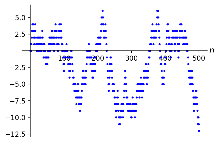
It is also nice to link this back to Equation 5.11–Equation 5.13: if the game is fair, then your expected accumulated profit at any point in time is $0$. Of course, you’ll win some and loose some, you may have a lucky streak in which you win quite a few one after the other even, yet ultimately (i.e. at larger time scales) such a lucky streak will always be compensated for by negative streaks. As discussed below Equation 5.11: a “typical” path of the process i.e. a typical realisation of such a (long, even never ending!) evening in the casino will see your accumulated profit over time fluctuate around the level $\mu=\E[X_0]=\E[X_1]=\ldots$ i.e. in this case $\mu=0$. If the game is unfair in your disadvantage i.e. $\E[Y]<0$, then Equation 5.13 shows that your expected accumulated profit will (strictly in this case) decrease over time, and though you may still very well have lucky streaks and reach high levels of accumulated profit, inevitably in the long run your luck is going to run out i.e. on large enough timescales a “typical” path will show a downwards trend.

These thoughts of what happens to our process in the long run can also be reinforced by looking at the good old (strong) law of large numbers (see e.g. Wiki): \[\frac{1}{n} X_n \stackrel{\text{a.s.}}{\longrightarrow} \E[Y] \quad \text{as $n \to \infty$} \tag{5.15}\] (recall the concept of almost sure convergence from Section 2.7, where in this case we have convergence to a constant random variable). If $\E[Y]>0$ (i.e. the strict submartingale case) then due to the presence of the $1/n$ term, it follows that $X_n \stackrel{\text{a.s.}}{\longrightarrow} \infty$ and the analogue if $\E[Y]<0$ (i.e. the strict supermartingale case). If $\E[Y]=0$ i.e. the martingale case, then a “typical” path of our process will fluctuate around the level $0$ as mentioned before, and in fact ever more “wild” i.e. with higher positive peaks and lower negative valleys as time increases, but Equation 5.15 shows that the positive and negative values achieved by these peaks/valleys nevertheless grow slow enough that after multiplication by $1/n$ the result still converges to $0$.

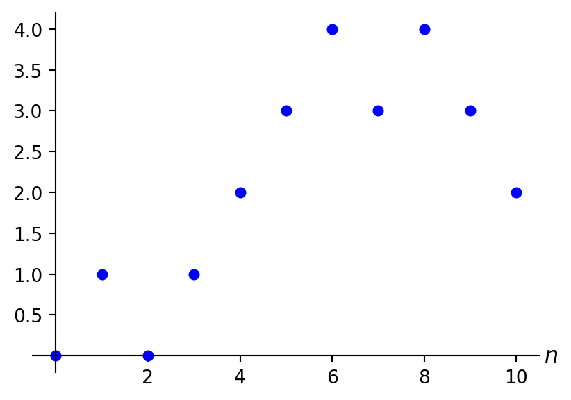
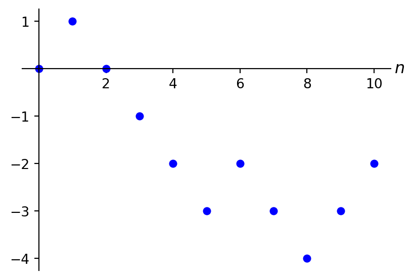
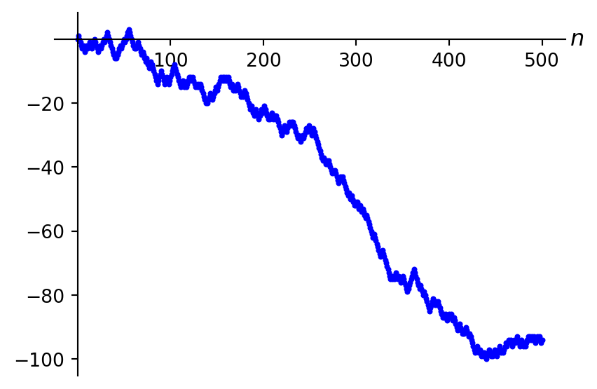
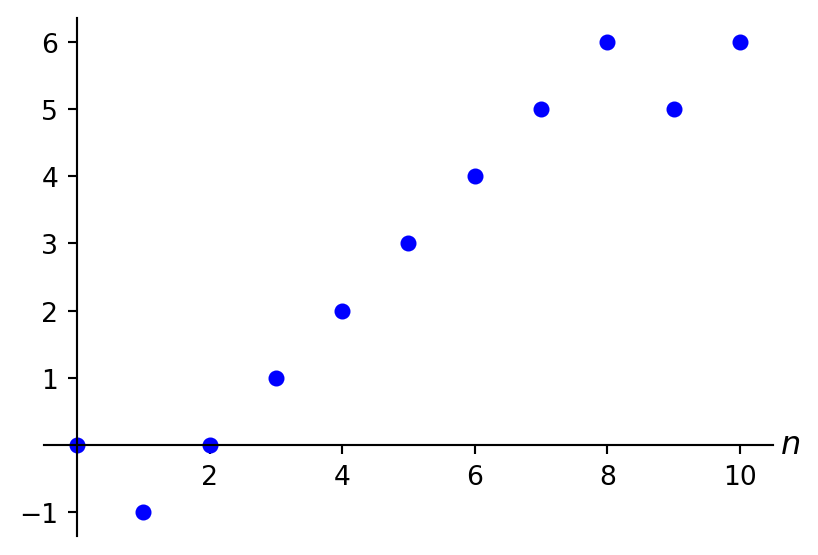
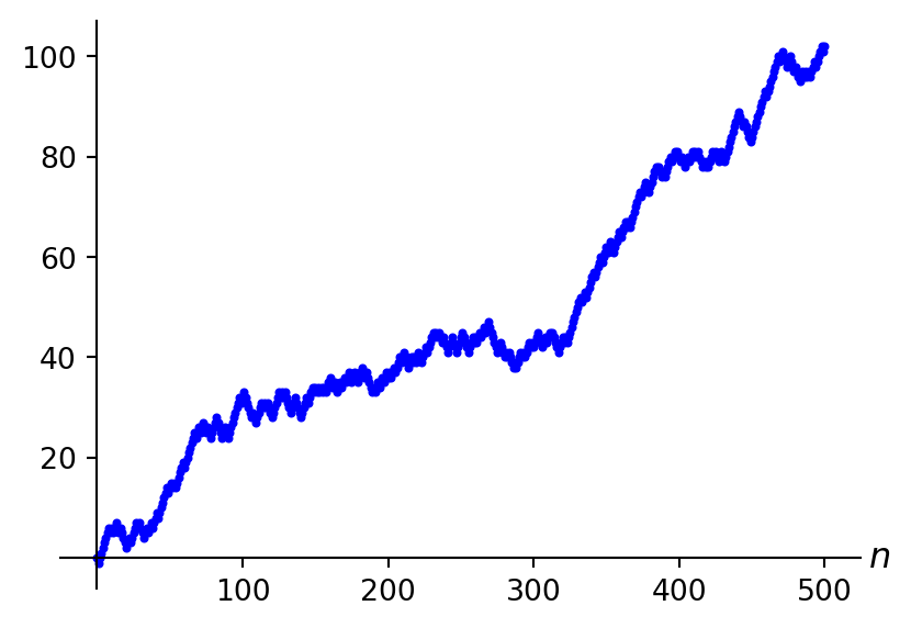
To make the behavious discussed above a bit more insightful, consider the special case that the game has only two possible outcomes: your profit is either $1$ or $-1$ i.e. $Y$ takes only the values $1$ and $-1$, say with probabilities $p \in [0,1]$ and $1-p$. As you can readily check by working out $\E[Y]$, in this case $(X_n)_{n=0,1,\ldots}$ is a (strict) supermartingale resp. martingale resp. (strict) submartingale if and only if $p \in [0,1/2)$ resp. $p=1/2$ resp. $p \in (1/2,1]$.

Further in this situation, starting with a profit of $0$ at time $n=0$ and then going forward by always adding either $-1$ or $1$ to our accumulated profit at each time step, our accumulative profits process only “visits” the integers $\Z=\{\ldots,-2,-1,0,1,2,\ldots\}$. In this case our process is known as a simple random walk.

You can find some simulated paths in Figure 5.2 — have a good look through these and make for yourself the link back to what we discussed above!

(a) Short timescale with $p=1/2$ i.e. the martingale case. You win some, you lose some

Exercises

You can now do Exercise 5.3–Exercise 5.5.

5.4 A simple betting/investment model

As mentioned in Section 5.1, one of the many important applications of martingales is in financial mathematics in a broad sense — be it for an evening in a casino or for advanced trading on the financial markets. We won’t dwell on that too much in this course (there’s dedicated courses for modelling financial markets etc.), but it is useful to discuss some small aspect of that, both to get some feel for this but also because it comes in handy in some proofs in the remainder of this chapter!

In the example Example 5.3 we saw some first examples of (sub/super)martingales by considering the evolution of accumulated profits from playing the same game repeatedly. Let’s now slightly extend that model by giving the player the option to vary how much money they put into each game i.e. their stake per game. To accomodate this, let’s define \[Y:=\text{profit from the game per £1 stake}.\] So, for every £1 you bet on the game you get back $£(Y+1)$, so that $Y=0$, $Y<0$, $Y>0$ resp. represents the situation that you break even, lose money, make money resp. For your typical game, the payout just gets scaled up with how much you put in (otherwise it doesn’t make a lot of sense to talk about “per £1 stake”), i.e. if $Y=5$ then you make a profit of £5 for each £1 that you put in, so if your stake was £10 then you have made a neat profit of £50. In general, if your stake is $c$, then after the game you are $cY$ wealthier (or poorer eh!).

To accommodate playing such a game repeatedly, take some probability space $(\Omega,\mathcal{F},\P)$ on which this $Y$ is a random variable, and let $Y_1, Y_2, \ldots$ be independent copies of $Y$. Assume that they are integrable. We create a filtration $(\mathcal{F}_n)_{n=0,1,\ldots}$ by setting \[\mathcal{F}_0=\{\emptyset,\Omega\} \quad \text{ and } \quad \mathcal{F}_n=\sigma(Y_1,\ldots,Y_n) \quad \text{for all } n=1,2,\ldots, \tag{5.16}\] so at any time $n=1,2,\ldots$ we have played and know the result of the first $n$ games. Now we would like to allow a player to vary their stake per game, let’s write $C_n$ for their stake in the $n$-th game (at time $n=0$ nothing has happened yet). Naturally, a player needs to decide on their stake for the $n$-th game before time $n$ when the result of that game becomes known, but they should be able to use the information up until time $n-1$ i.e. from the first $n-1$ games (for instance to be able to compute how much money they have left after the first $n-1$ games!). That is to say, it is natural to demand that for every $n=1,2,\ldots$, $C_n$ is $\mathcal{F}_{n-1}$-measurable. Think about it as follows: at every time $n=1,2,\ldots$, you learn first the result of the $n$-th game i.e. the value of $Y_n$ and you must then also immediately decide your stake for the next game.

From a stochastic processes perspective, we call this property previsibility:

Definition 5.3 On some filtered probability space $(\Omega,\mathcal{F},(\mathcal{F}_n)_{n=0,1,\ldots},\P)$, a stochastic process $(C_n)_{n=1,2,\ldots}$ (note that there is no $C_0$) is called previsible if $C_n$ is $\mathcal{F}_{n-1}$-measurable for all $n=1,2,\ldots$.

So such a previsible process $(C_n)_{n=1,2,\ldots}$ represents a “betting strategy” if you will, and it naturally comes with an associated accumulated profits process $(X_n)_{n=0,1,\ldots}$ given by \[X_0=0 \quad \text{ and } \quad X_n=\sum_{i=1}^n C_i Y_i \quad \text{for all } n=1,2,\ldots \tag{5.17}\] which gives the accumulated profit at any time $n=0,1,\ldots$. Note that $(X_n)_{n=0,1,\ldots}$ is adapted to the filtration we’ve created in Equation 5.16, because for every $n=1,2,\ldots$ $X_n$ is a function of $C_1, \ldots, C_n$ and $Y_1, \ldots, Y_n$ which are all $\mathcal{F}_n$-measurable random variables and hence $X_n$ is $\mathcal{F}_n$-measurable as well. Further, from the perspective of our interpretation, only non-negative random variables $C_n$ really make sense, but for the purely mathematical construct we may just as well consider general real valued ones.

Now, coming from Example 5.3 (note that we find the simpler accumulated profits process from that example back if we simply choose $C_n=1$ for all $n=1,2,\ldots$ in Equation 5.17), a natural question to ask is whether the introduction of such a betting strategy makes any difference. For instance, if we’re playing fair games i.e. with $\E[Y]=0$ then we saw in Example 5.3 that with $C_n=1$ for all $n=1,2,\ldots$ the accumulated profits process is a martingale. Is it possible, with the extra freedom of being able to choose a betting strategy, to do any better e.g. to create a submartingale (which “increases on average”)?

Maybe surprisingly, but the answer is no. At least under some mild conditions to keep things integrable, there is no escaping the martingale behaviour, no matter how smart you try to be with your betting strategy! So if nothing else, at least you can take this with you for when you next go home to your family and meet that annoying uncle Hank who claims he has developed this very smart strategy allowing him to make money from a casino etc. ;).

This is not very hard to see. We have already seen that $(X_n)_{n=0,1,\ldots}$ is adapted, so it remains to check integrability and the martingale property (cf. Definition 5.2). Assuming that $(C_n)_{n=1,2,\ldots}$, besides previsible, is also an integrable process and that $C_1 Y_1, C_2 Y_2, \ldots$ are all integrable, we get from the triangle inequality and the linearity property of expectations (cf. Proposition 3.6 i) that for any $n=1,2,\ldots$ \[\begin{align*} \E[\lvert X_n \rvert] &= \E \left[ \left\lvert \sum_{i=1}^n C_i Y_i \right\rvert \right] \\ &\leq \E \left[ \sum_{i=1}^n \lvert C_i Y_i \rvert \right] \\ &=\sum_{i=1}^n \E \left[ \lvert C_i Y_i \rvert \right] \\ &< \infty, \end{align*} \] the final step because we assumed that $\E [ \lvert C_i Y_i \rvert ]<\infty$ for all $i=1,2,\ldots$. If you prefer a sufficient condition only on $(C_n)_{n=1,2,\ldots}$, then you could for instance take the condition that each random variable $C_n$ is bounded i.e. that for any $n=1,2,\ldots$ a constant $c_n$ exists so that $\lvert C_n \rvert \leq c_n$ (pointwise)². Indeed then, using the well known $\lvert ab \rvert \leq \lvert a \rvert \lvert b \rvert$: \[\begin{align*} \E \left[ \lvert C_n Y_n \rvert \right] &\leq \E \left[ \lvert C_n \rvert \lvert Y_n \rvert \right] \\ &\leq \E \left[ c_n \lvert Y_n \rvert \right] \\ &\leq c_n \E \left[ \lvert Y_n \rvert \right] \\ &<\infty, \end{align*} \] where the second inequality uses non-negativity (cf. Proposition 3.6 ii), the third linearity (cf. Proposition 3.6 i), and the final one that $Y_n$ is by assumption integrable.

² For clarity: note that what this means is that the range of the random variable $C_n$ i.e. the set of its possible values in $\R$ (recall from Section 2.2) is contained in the interval $[-c_n,c_n]$, for some (finite) $c_n$. This is not trivially always true, think for example about a random variable with a Poisson distribution so that its range is $\{0,1,\ldots\}$ (no finite upperbound) or with a Normal distribution so that its range is the whole of $\R$ (so neither a lower nor an upperbound)

For the martingale property, using the formulation from Exercise 5.3 (which is typically handy when dealing with a summation form), we have for any $n=0,1,\ldots$ that $X_{n+1}-X_n=C_{n+1} Y_{n+1}$ and hence \[\begin{align*} \E[X_{n+1}-X_n \, | \, \mathcal{F}_n] &= \E[C_{n+1} Y_{n+1} \, | \, \mathcal{F}_n] \\ &= C_{n+1} \E[Y_{n+1} \, | \, \mathcal{F}_n] \\ &= C_{n+1} \E[Y_{n+1} ] \\ &= C_{n+1} \E[Y ], \end{align*} \] where the second equality uses the “taking out what is known” property of conditional expectations, cf. Theorem 4.2 v (recall that $(C_n)_{n=1,2,\ldots}$ is assumed to be previsible), the third that $Y_{n+1}$ is independent of $Y_1, \ldots, Y_n$ and hence of $\mathcal{F}_n$ (cf. Equation 5.16), and the final one that $Y_1, Y_2, \ldots$ are all (independent) copies of $Y$. So we see that, indeed, $(X_n)_{n=0,1,\ldots}$ is a martingale if $\E[Y]=0$. Further, under the extra assumption that $(C_n)_{n=1,2,\ldots}$ is a non-negative process, we also immediately see from the above that $(X_n)_{n=0,1,\ldots}$ is a sub- resp. supermartingale if $\E[Y] \geq 0$ resp. $\E[Y] \leq 0$.

Proposition 5.1 Let $Y$ be an integrable random variable on some probability space $(\Omega,\mathcal{F},\P)$ and let $Y_1, Y_2, \ldots$ be independent copies of $Y$. Define the filtration by Equation 5.16. For any previsible process $(C_n)_{n=1,2,\ldots}$ (cf. Definition 5.3), define the process $(X_n)_{n=0,1,\ldots}$ as in Equation 5.17.

Assume that for every $n=1,2,\ldots,$ a constant $c_n$ exists so that $\lvert C_n \rvert \leq c_n$ (pointwise). Then:

if $\E[Y]=0$, $(X_n)_{n=0,1,\ldots}$ is a martingale,
if in addition $(C_n)_{n=1,2,\ldots}$ is a non-negative process, then $(X_n)_{n=0,1,\ldots}$ is a submartingale resp. supermartingale if $\E[Y] \geq 0$ resp. $\E[Y] \leq 0$.

Finally in this section, as we all know it’s only a small step from betting to trading on a financial market ;) — indeed the setup above is with a small reformulation only also quite suited as a simple investment model.

Imagine some publicly traded financial instrument, say a stock of some company. Say that every day at 5pm, the value of (one unit of) the stock at that point in time becomes known, and let’s denote/model this value by $Y_n$ for day $n=0,1,\ldots$, where $(Y_n)_{n=0,1,\ldots}$ is an adapted stochastic process on some filtered probabilty space $(\Omega,\mathcal{F},(\mathcal{F}_n)_{n=0,1,\ldots},\P)$. Note that, contrary to the betting example above, in this situation $Y_0, Y_1, \ldots$ are typically not (mutually) independent random variables — for instance, the probability that the value at day $n$ is more than £100 is much larger if at day $n-1$ the value is say £90 than if the value is say £5 no?

As investor, on the evening of day $0$ you decide to buy $C_1 \in \R$ units of the stock for the then current value of $Y_0$. You may well choose $C_1=0$ i.e. not buy at all, and you can even choose $C_1<0$ which seems strange if you’re new to this but it is generally a valid thing to do (called short selling). We assume for simplicity that you can buy any number of units that you want, and that there are no extra costs (no transaction costs for instance) involved in doing so. So in the evening of day $0$ you spend $C_1 Y_0$ i.e. have a profit of $-C_1 Y_0$.

Then, on the evening of day 1, when the new value $X_1$ is known, you sell your $C_1$ units of stock which makes you $C_1 Y_1$ and so you conclude this first trading cycle with a profit (positive or negative) of $C_1 Y_1-C_1 Y_0=C_1(Y_1-Y_0)$. After selling, on that same evening you decide how many units you want to buy for the next trading cycle, say $C_2$, at a cost of $C_2 Y_1$. (Obviously you could do that first selling and then buying together in one single transaction, but it’s easier as first explanation to see them as separate transactions.)

Repeating this nice relaxing evening hobby day after day, after you have concluded the $n$-th trading cycle (so after the selling on day $n$ but before the buying — if any) you have obtained an accumulated profit of $X_n$, where \[X_0=0 \quad \text{and} \quad X_n = \sum_{i=1}^n C_i(Y_i-Y_{i-1}) \quad \text{for $n=1,2,\ldots$.} \tag{5.18}\] Very similar to the above betting-on-games story, the accumulated profit at time $n$ here is the sum of $n$ repeated investments/bets, and note that analogue to above, to make it an interesting/non-trivial activity, you need to decide on a value for $C_i$ before you know the value of $Y_i$ (but the money you make from that decision does depend on $Y_i$) i.e. only using the values of $Y_0,\ldots,Y_{i-1}$ i.e. your investment strategy $(C_n)_{n=1,2,\ldots}$ must again be previsible (cf. Definition 5.3). What is different from the betting-on-games story is that we have moved from i.i.d. random variables modelling the profit per £1 stake in the games, to these differences (or increments as we like to call them) $Y_1-Y_0, Y_2-Y_1, \ldots$ in Equation 5.18 that model the day-to-day changes in the value of a unit of the stock.

Despite that difference though, we can prove very similar conclusions as in Proposition 5.1 (the proof is all yours in Exercise 5.6):

Proposition 5.2 Let $(Y_n)_{n=0,1,\ldots}$ be a stochastic process on some filtered probabilty space $(\Omega,\mathcal{F},(\mathcal{F}_n)_{n=0,1,\ldots},\P)$. Let $(C_n)_{n=1,2,\ldots}$ be a previsible process (cf. Definition 5.3) with the property that for every $n=1,2,\ldots$, a constant $c_n$ exists so that $\lvert C_n \rvert \leq c_n$ (pointwise). Finally let $(X_n)_{n=0,1,\ldots}$ be as defined in Equation 5.18.

Then we have the following.

If $(Y_n)_{n=0,1,\ldots}$ is a martingale, then $(X_n)_{n=0,1,\ldots}$ is also a martingale.
If $(Y_n)_{n=0,1,\ldots}$ is a submartingale resp. supermartingale and $(C_n)_{n=1,2,\ldots}$ is a non-negative process, then $(X_n)_{n=0,1,\ldots}$ is also a submartingale resp. supermartingale.

Remark 5.2.

Note that Proposition 5.2 has a similar interpretation as we saw for bettng in Proposition 5.1: if the value process of the unit stock is a (super)martingale i.e. on average tends to fluctuate around a constant level or tends to decrease, then there is no smart choice for an investment strategy possible that turns the accumulated profit process into a strict submartingale (i.e. a process that on average tends to strictly increase) for instance.
These accumulated profit processes for individual investors are a core tool in mathematical finance — there is a lot more to be said about them but as mentioned above already, we’ll leave that for dedicated financial maths courses.
The accumulated profits process Equation 5.18 has many important uses (and not just in this specific investment interpretation — in fact we’ll see one in the next section). In general it is called a martingale transform, and it is the discrete time form of a stochastic integral (as you may well encounter in other courses!).
Note that we can see the betting-on-games story from above as a special case of the investment model: given the i.i.d. random variables $Y_1, Y_2, \ldots$ denoting the profits per game per £1 stake, consider the process $(Z_n)_{n=0,1,\ldots}$ given by \[Z_0=0 \quad \text{and} \quad Z_n=\sum_{i=1}^n Y_i \quad \text{for all } n=1,2,\ldots\] i.e. the accumulated profits process if you were to put a stake of £1 into each game.

Then if we interpret $(Z_n)_{n=0,1,\ldots}$ as the evolution of the (unit) price of some stock in which we can invest, then picking a strategy i.e. previsible process $(C_n)_{n=1,2,\ldots}$, the accumulated profit process $(X_n)_{n=0,1,\ldots}$ from the investment Equation 5.18 boils down to $X_0=0$ and for all $n=1,2,\ldots$ \[X_n = \sum_{i=1}^n C_i(Z_i-Z_{i-1}) = \sum_{i=1}^n C_i Y_i\] i.e. it also equals the accumulated profits process for the playing the games (cf. Equation 5.17)!

Exercises

You can now do Exercise 5.6.

5.5 Doob’s decomposition theorem

This section is the first of several dedicated to discussing a suite of beautiful, fundamental and very important results for martingales all (mostly) due to the mathematician Joseph Doob, an iconic figure in the field!

We don’t use anything from the previous section on the simple investment model other than the notion of a previsible process from Definition 5.3. Rather we get our inspiration from a little bit further back: Section 5.3 and also Example 5.3. Recall that in Example 5.3 we saw nice explicit examples of a sub- and supermartingale. Looking again a bit closer at the examples of paths we saw there, then as discussed these showed some “fluctuating” martingale like behaviour but rather than fluctuating around a constant level like a martingale does, it seemed to be fluctuating around an increasing (resp. decreasing) function, like a trend line really. That raises the question whether there is maybe a way to “decompose” a sub- or supermartingale into a fluctuating martingale part and a “trend” part, analogue in spirit to how a function $f(t)=at+\sin(t)$ decomposes into a fluctuating (around a constant level) part $t \mapsto \sin(t)$ and a trend $t \mapsto at$.

Ideally you would like such a decomposition, if it exists, to be unique. This requires that the martingale part and “trend” part are different classes of processes, in the sense that you shouldn’t be able to subtract a little bit of martingale from the martingale part and add that to the “trend” part to get another viable decomposition.

Now, as it turns out, the class of martingales and the class of previsible processes defined in Definition 5.3 have exactly this property of being different in this way. Indeed, if $(X_n)_{n=0,1,\ldots}$ is a stochastic process on some filtered probability space $(\Omega,\mathcal{F},(\mathcal{F}_n)_{n=0,1,\ldots},\P)$ that starts from $0$ (i.e. $X_0=0$) and that is both a martingale and previsible, look at what happens. The martingale property from Definition 5.2 tells us that for any $n=0,1,\ldots$ we have that $\E[X_{n+1} \, | \, \mathcal{F}_n]=X_n$. But by the previsibility property from Definition 5.3, $X_{n+1}$ is $\mathcal{F}_n$-measurable and hence by Theorem 4.2 ii we have that $\E[X_{n+1} \, | \, \mathcal{F}_n]=X_{n+1}$. So it follows that $X_{n+1}=X_n$ (a.s., to be precise, due to the use of conditional expectations). Since this holds for any $n=0,1,\ldots$ and $X_0=0$, we in fact get that $X_n=0$ a.s. for all $n=0,1,\ldots$. This implies even the (seemingly) slightly stronger statement that (recall from Exercise 2.5) \[X_n=0 \quad \text{for all }n=0,1,\ldots \text{ (a.s.)}. \tag{5.19}\] So, the only process that starts from $0$ and is both a martingale and previsible is the trivial process that is (a.s.) constantly equal to $0$!

This, admittedly slightly leading ;), introduction is aiming to out you on the track of thinking that it might make sense to investigate whether we can decompose a sub- or supermartingale in a unique way in a martingale part and a previsible part. That turns out to be the case, and not only for sub- and supermartingales but even for any process!

Theorem 5.1 (Doob’s decomposition theorem) Let $(X_n)_{n=0,1,\ldots}$ be an adapted and integrable process on some filtered probability space $(\Omega,\mathcal{F},(\mathcal{F}_n)_{n=0,1,\ldots},\P)$ (cf. Definition 5.1). Then we have the following.

We can decompose $(X_n)_{n=0,1,\ldots}$ as follows: \[X_n=X_0+M_n+A_n \quad \text{for all }n=0,1,\ldots \quad \text{(a.s.),} \tag{5.20}\] where $(M_n)_{n=0,1,\ldots}$ is a martingale starting from $0$ (i.e. $M_0=0$), and $(A_n)_{n=0,1,\ldots}$ is an integrable and previsible process starting from $0$.

This decomposition is unique in the sense that for any other choice of processes, say $(M_n')_{n=0,1,\ldots}$ and $(A_n')_{n=0,1,\ldots}$, fitting the role of $(M_n)_{n=0,1,\ldots}$ and $(A_n)_{n=0,1,\ldots}$ above we have that \[M_n'=M_n \text{ for all }n=0,1,\ldots \text{ (a.s.)}\quad \text{and} \quad A_n'=A_n \text{ for all }n=0,1,\ldots \text{ (a.s.).}\]
$(X_n)_{n=0,1,\ldots}$ is a submartingale if and only if in the above decomposition, the process $(A_n)_{n=0,1,\ldots}$ is non-decreasing in the sense that $A_n \leq A_{n+1}$ for all $n=0,1,\ldots$ a.s. (The obvious analogue for supermartingales also holds).

Proof. The proof is actually not very difficult, just a bit of work to get it all sorted.

Let’s start with part i. Where do you start with something like this? Well, essentially what we need to do is figure out what part/process we need to subtract from $(X_n)_{n=0,1,\ldots}$ so that the remainder is a martingale, and hopefully that process we subtracted is then indeed previsible. Ok. What makes a general (adapted and integrable) process $(X_n)_{n=0,1,\ldots}$ not a martingale? Well the fact that martingale property (cf. Definition 5.2) does not hold in general i.e. that $\E[X_{n+1} \, | \, \mathcal{F}_n] \not= X_n$. Alright, but what if we then simply collect the differences between these two terms in the part that we subtract, then the remainder should have the martingale property no? That works!

Define $(A_n)_{n=0,1,\ldots}$ as \[A_0:=0, \quad A_n := \sum_{k=0}^{n-1} \big( \E[X_{k+1} \, | \, \mathcal{F}_k] -X_k \big) \quad \text{ for all } n=1,2,\ldots. \tag{5.21}\] Be aware that also here our slight ambiguity of working with conditional expectations comes to hunt us once more (cf. Definition 4.2): it means that $A_n$ is not defined pointwise but only on an almost sure event. As always, we don’t care what happens on the complement of that event but it does explain the “a.s.” qualifier in Equation 5.20. Now, since conditioning on $\mathcal{F}_k$ results in an $\mathcal{F}_k$-measurable random variable (recall from Definition 4.2), for every $k=0,\ldots,n-1$ the difference $\E[X_{k+1} \, | \, \mathcal{F}_k] -X_k$ is $\mathcal{F}_k$-measurable (cf. Proposition 2.1 iv) and, since the $\sigma$-algebras in a filtration are non-decreasing (cf. Definition 5.1), also all $\mathcal{F}_{n-1}$-measurable. So $A_n$, as a sum of $\mathcal{F}_{n-1}$-measurable random variables, is itself also $\mathcal{F}_{n-1}$-measurable (again by Proposition 2.1 iv). So that is the previsibility of $(A_n)_{n=0,1,\ldots}$ sorted.

To see that $(A_n)_{n=0,1,\ldots}$ is integrable is a matter of using the triangle inequality and linearity of expectations in a very similar way as in Exercise 5.6. The only new element that we need here is that for any $k=0,1,\ldots$ we can write \[\begin{aligned} \E \big[ \big\lvert \E[X_{k+1} \, | \, \mathcal{F}_k] \big\rvert \big] &\leq \E \big[ \E[\lvert X_{k+1} \rvert \, | \, \mathcal{F}_k] \big] \\ &= \E[\lvert X_{k+1} \rvert] \\ &<\infty, \end{aligned} \] where the first inequality uses non-negativity of conditional expectations (cf. Theorem 4.1 ii) since $X_{k+1} \leq \lvert X_{k+1} \rvert$ — or use Jensen’s inequality for conditional expectations (cf. Theorem 4.1 iv) with $f(x)=\lvert x \rvert$ — together with the non-negativity property of expectations, cf. Proposition 3.6 ii; the equality uses Theorem 4.2 i; and the final inequality uses that $(X_n)_{n=0,1,\ldots}$ is by assumption integrable.

To complete the first statement (besides the uniqueness), we have now defined what we think our choice for $(A_n)_{n=0,1,\ldots}$ should be, and it remains to show that the process $(M_n)_{n=0,1,\ldots}$ defined as (so as to make Equation 5.20 indeed work) \[M_n:=X_n-X_0-A_n \quad \text{for all } n=0,1,\ldots \tag{5.22}\] is indeed a martingale starting from $0$. Since $A_0=0$, it is immediate that $M_0=0$. To see that it is integrable, just apply the triangle inequality to the right hand side of Equation 5.22 and use that all terms have finite expectation (because both $(X_n)_{n=0,1,\ldots}$ and $(A_n)_{n=0,1,\ldots}$ are integrable). To see the martingale property, using Exercise 5.3 we can write for any $n=0,1,\ldots$ \[\begin{aligned} \E[M_{n+1}-M_n \, | \, \mathcal{F}_n] &= \E[X_{n+1}-X_n-A_{n+1}+A_n \, | \, \mathcal{F}_n] \\ &= \E[X_{n+1} \, | \, \mathcal{F}_n] -X_n-A_{n+1}+A_n \\ &= \E[X_{n+1} \, | \, \mathcal{F}_n] -X_n- \big( \E[X_{n+1} \, | \, \mathcal{F}_n] -X_n \big) \\ &=0, \end{aligned} \] where we just plug in Equation 5.22; use linearity; use the fact that $X_n$, $A_n$ and $A_{n+1}$ are all $\mathcal{F}_n$-measurable (recall that $(A_n)_{n=0,1,\ldots}$ is previsible) so that we can apply Theorem 4.2 ii; and finally just plug in Equation 5.21. Of course this is all just light algebra around the key fact that we defined $(A_n)_{n=0,1,\ldots}$ exactly to make this work out!

Finally for part i, to prove the uniqueness claim, if $(M_n')_{n=0,1,\ldots}$ and $(A_n')_{n=0,1,\ldots}$ are alternative choices for the decomposition, then it follows from Equation 5.20 that \[M_n-M_n'=A_n-A_n' \quad \text{for all }n=0,1,\ldots \text{ (a.s.)}.\] But the left hand side, being the difference of two martingales starting from $0$, is again a martingale starting from $0$ as you can easily check from Definition 5.2. The right hand side is previsible since both $(A_n)_{n=0,1,\ldots}$ and $(A_n')_{n=0,1,\ldots}$ are (as you can readily check from Definition 5.3). So the process $(M_n-M_n')_{n=0,1,\ldots}$ is a previsible martingale starting from $0$, and as we discussed above the statement of this theorem (cf. Equation 5.19), this indeed means that \[M_n=M_n' \quad \text{for all }n=0,1,\ldots \text{ (a.s.)}.\]

Finally finally ;), we need to look at part ii of the theorem. The good news is that this is pretty obvious. We see from Equation 5.21 that for all $n=0,1,\ldots$ that \[\E[X_{n+1} \, | \, \mathcal{F}_n] -X_n \geq 0 \text{ (a.s.)} \iff A_{n+1}-A_n \geq 0 \text{ (a.s.)}.\] So the submartingale property holds if and only if for each $n=0,1,\ldots$, $A_{n+1} \geq A_n$ a.s., and now again use Exercise 2.5 to get the exact statement from the theorem.

In this course we won’t make use of this result a lot. Nevertheless it is a fundamental result in many areas where martingales are used, for instance in mathematical finance. It also underlines just how natural martingales come into the picture as fundamental building blocks of stochastic processes!

Let’s conclude with seeing how this all works out in Example 5.3, from which we also borrowed some visuals to introduce/motivate this result:

Example 5.4 Let’s have a look back at Example 5.3, where we play the same game with profit distribution $Y$ infinitely often (independently), with profit per game $Y_1, Y_2, \ldots$ (independent copies of $Y$), and the accumulated profit given by the process $(X_n)_{n=0,1,\ldots}$ expressed as \[X_0:=0 \quad \text{ and } \quad X_n=\sum_{i=1}^n Y_i \quad \text{for all } n=1,2,\ldots.\]

Let’s see if we can figure out for this process what its martingale and previsible parts are! Of course our proof above was constructive i.e. we actually showed what the previsible part $(A_n)_{n=0,1,\ldots}$ looks like in Equation 5.21, so let’s just start there: \[A_0:=0, \quad A_n := \sum_{k=0}^{n-1} \big( \E[X_{k+1} \, | \, \mathcal{F}_k] -X_k \big) \quad \text{ for all } n=1,2,\ldots.\] Further we had already seen in Equation 5.14 that for any $n=0,1,\ldots$ \[\E[X_{n+1}-X_n \, | \, \mathcal{F}_n]=\E[Y]\] which means that our previsible part takes the very simple form \[A_n = \sum_{k=0}^{n-1} \E[Y] = n \E[Y] \quad \text{for all } n=0,1,\ldots. \tag{5.23}\] It is a rather trivial example of a stochastic process: it is simply a deterministic function of $n$ (i.e. each $A_n$ is a constant random variable).

Applying part ii of Theorem 5.1 confirms what we had already checked by direct computation in Example 5.3: $(X_n)_{n=0,1,\ldots}$ is a submartingale resp. martingale resp. supermartingale if and only if $\E[Y] \geq 0$ resp. $\E[Y]=0$ resp. $\E[Y] \leq 0$. (If you’re not sure how to see the martingale statement from only part ii of that theorem, just observe from Definition 5.2 that a process is a martingale if and only if it is both a sub- and supermartingale).

It’s also interesting to see what the martingale part of $(X_n)_{n=0,1,\ldots}$ looks like: \[M_n = X_n-A_n = \sum_{i=1}^n Y_i - n \E[Y] = \sum_{i=1}^n (Y_i-\E[Y]) \quad \text{for all } n=0,1,\ldots.\] Adding that final step shows that this has a very nice interpretation: the martingale part can still be seen as the accumulated profit after $n$ games, but since \[\E \big[ Y_i-\E[Y] \big] = \E[Y_i]-\E[Y]=0\] the games are now fair! What happens here is basically the following. Suppose that you play a game in a casino where you’re expected to lose £10 per game. You put the money you have on your table (which can be a negative amount as well). You also open a line of credit with the casino. Each time before you play the game, you borrow £10 from the casino and add that to the money on your table. With this extra income, the games you play are fair. Your accumulated profit after $n$ games is now the sum of the money on your table (the result of playing $n$ fair games i.e. the martingale part) plus the “profit” from your debt i.e. $-10n$ (the previsible part). Of course, this line of credit business has no actual effect on your actual accumulated profit, it’s just an accounting trick if you will that splits your income/outgo stream into a stream coming from fair games and a previsible (even deterministic) stream that reflects the difference in expected profit between the games you are actually playing and fair ones.

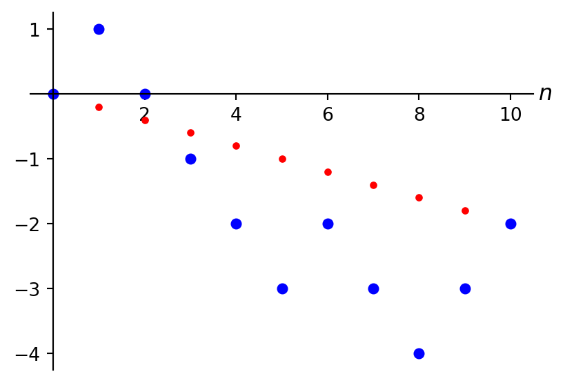
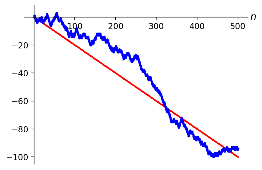
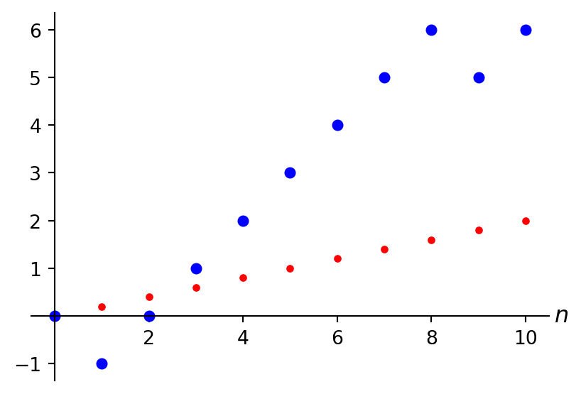
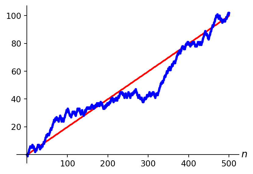
Finally, we mentioned at the start of this section a visual interpretation of this decomposition: the original process as consisting of a “trend” (as we know now, a previsible process) part plus a martingale part “fluctuating” around the constant level $0$. Figure 5.3 shows the paths of $(X_n)_{n=0,1,\ldots}$ again we previously already saw in plots (c)–(f) in Figure 5.3, but now with the relevant path of $(A_n)_{n=0,1,\ldots}$ added in red (simply using Equation 5.23 of course). Note how the longer time scale plots nicely confirm this visual idea!

Keep in mind though that this is a special case, where $(A_n)_{n=0,1,\ldots}$ is a deterministic function, even a linear one. This is of course due to some very nice homogeneity properties that our process $(X_n)_{n=0,1,\ldots}$ has in this example — in general $(A_n)_{n=0,1,\ldots}$ will be an actual stochastic process!

(a) Cf. Figure 5.2 (c): $p=0.4$ and hence $\mathbb{E}[Y]=-0.2$

5.6 Doob’s martingale convergence theorem

We conclude this chapter with yet another seminal result from our new hero Doob!

Let’s have another look at Doob’s decomposition theorem Theorem 5.1, which tells us roughly speaking that a process can be decomposed into a fluctuating (martingale) part and a trend (previsible) part. Could a path of such a process $(X_n)_{n=0,1,\ldots}$ i.e. the sequence of real numbers $X_0(\omega), X_1(\omega), \ldots$ possibly have a finite limit? Well, getting some inspiration from the plots in Figure 5.3 (b) & (d), these do seem to show convergence but only to $-\infty$ (supermartingale case) and $\infty$ (submartingale case) so not something finite sadly. For the martingale case, looking at Figure 5.2 (b), it is maybe not so obvious from that plot but if you would take even longer timescales, you’d see that the peaks resp. valleys get only higher resp. deeper as time goes on, so in that case we have no convergence at all!

However, on the other hand, it’s also not hard to imagine that there are situations in which there is a finite limit. In Figure 5.3 (b) & (d) for instance, if we would change the ingredients of the corresponding example a little bit so that the red trend line would converge to some finite limit and the fluctuating around it by the blue path would gradually dampen out as time progresses then there would be a finite limit indeed.

The goal of this section is to formulate conditions under which a finite limit is guaranteed to exist (well, almost surely at least). This result is called the martingale convergence theorem, arguably one of the most important results in the field with a lot of important consequences and applications!

Before carrying on, recall the following two key facts about a sequence of real numbers $a_0, a_1, \ldots$:

Fact 1: if the sequence is monotone (i.e. either non-decreasing or non-increasing) then it has a limit (it may be $\pm\infty$ though). See e.g. Wiki if you’d like a refresher about this.
Fact 2: in general it always holds that \[\liminf_{n \to \infty} a_n \leq \limsup_{n \to \infty} a_n,\] and the sequence has a limit if and only if \[\liminf_{n \to \infty} a_n = \limsup_{n \to \infty} a_n\] in which case the limit is equal to this limsup and/or liminf (which may be $\pm\infty$). See e.g. Remark 3.5 in which we discussed this in more detail.

The key idea behind the martingale convergence theorem is to link convergence of a sequence of real numbers to the number of upcrossings of any interval it can make. Fix some $\omega \in \Omega$ and consider the corresponding path $X_0(\omega), X_1(\omega), \ldots$ (so sequence of real numbers) of a process $(X_n)_{n=0,1,\ldots}$. We say that the path makes an upcrossing of $[a,b]$ between times $m_1$ and $m_2$ if \[X_{m_1}(\omega)<a; \quad X_n(\omega) \in [a,b] \text{ for all } m_1<n<m_2; \quad X_{m_2}(\omega)>b. \tag{5.24}\] We are particularly interested in the number of such upcrossings the path makes. We denote by $U_N^{a,b}(\omega) \in \{0,1,\ldots,N\}$ the number of upcrossings of $[a,b]$ the path makes up until time $N$ (i.e. we consider only $X_0(\omega), \ldots,X_N(\omega)$), and by \[U_\infty^{a,b}(\omega) := \lim_{N \to \infty} U_N^{a,b}(\omega) \in \{0,1,\ldots\} \cup \{\infty\} \tag{5.25}\] the number of upcrossings of $[a,b]$ the whole path makes — clearly $U_N^{a,b}(\omega)$ is non-decreasing in $N$, so this limit is well defined (cf. Fact 1 above) though it may well be $\infty$ of course.

Note that the above construction is on a pathwise (i.e. “per $\omega$”) basis, and hence what we have constructed here are mappings $U_N^{a,b}: \Omega \to \R$ and $U_\infty^{a,b}: \Omega \to \R \cup \{\infty\}$, indeed random variables (though for $U_\infty^{a,b}$ we have to let $\infty$ be part of the co-domain — remember that we have made some allowances for this in Chapter 3).

Intuitively it is not hard to see how the link between convergence and numbers of upcrossings works: for a path $X_0(\omega), X_1(\omega), \ldots$ to convergence to some limit, say we denote it by $V(\omega)$, as $n$ grows the $X_n(\omega)$’s must gradually ever get closer to $V(\omega)$ and hence in particular also closer to each other (if you’re in doubt, recall Cauchy sequences). Therefore if you take some $[a,b]$ not containing $V(\omega)$ then for $n$ large enough all $X_n(\omega)$’s are close enough to $V(\omega)$ so that they can’t be in $[a,b]$. If you take some $[a,b]$ that does contain $V(\omega)$ then for all $n$ large enough all $X_n(\omega)$’s are so close together that the maximal distance between any two of them is less than $b-a$. Either way we come to the following conclusion: for any interval $[a,b]$, there exists some time point (depending on the path i.e. $\omega$) after which there can be no more upcrossings of $[a,b]$, and hence in particular there can be only finitely many upcrossings of the interval. The converse is also true, and it is (even) enough to consider all rational $a$ and $b$ only (rather than all real ones):

Lemma 5.2 Fix some $\omega \in \Omega$. If for all $a,b \in \Q$ with $a<b$ we have that $U_\infty^{a,b}(\omega)<\infty$ then $\lim_{n \to \infty} X_n(\omega)$ exists (though it may be $\pm\infty$).

Proof. Denote \[i:=\liminf_{n \to \infty} X_n(\omega) \quad \text{and} \quad s:=\limsup_{n \to \infty} X_n(\omega).\] Recall from Fact 2 above that $i \leq s$. Suppose that we had $i<s$. Take $a,b \in \Q$ so that $i<a<b<s$ (this is possible since $\Q$ is dense in $\R$, recall the brief discussion in Proposition 1.2 iv for instance). Take some $m_1$ so that $X_{m_1}(\omega) <a$ (exists by def of the liminf). By def of the limsup, there exists an $m_2>m_1$ so that $X_{m_2}(\omega) >b$ and we have made an upcrossing. By def of the liminf, there exists an $m_3>m_2$ so that $X_{m_3}(\omega) <a$. You can reiterate this argument infinitely often, showing that there must be infinitely many upcrossings. But this is a contradiction with $U_\infty^{a,b}(\omega)<\infty$. So it cannot be true that $i<s$, and hence, by Fact 2 above, it must be the case that $i=s$ and that $\lim_{n \to \infty} X_n(\omega)$ exists.

So with this lemma in our pocket, we can shift our focus to finding conditions on $(X_n)_{n=0,1,\ldots}$ which guarantee that the number of upcrossings of any interval is finite. It’s probably not immediately clear to you that this would be any easier than the original problem though! Here a beautiful bit of creative thinking comes into play, where we also make use of the investment model we introduced in Section 5.4.

First, here is the intuitive idea. Interpret $(X_n)_{n=0,1,\ldots}$ as the evolution of a stock price as in Section 5.4. Fix any $a<b$ and consider an investment strategy as follows: wait until the stock price falls below $a$ and buy one unit of stock. Hold it until the price gets above $b$ and then sell it (so you collect a profit of at least $b-a$). Rinse and repeat. If there are infinitely many upcrossings, then you would ultimately become infinitely wealthy i.e. the accumulated profits process associated with this strategy would ultimately reach arbitrarily high levels no? But we know from Proposition 5.2 that if $(X_n)_{n=0,1,\ldots}$ is a (super)martingale, then the accumulated profits process (for any (previsible) strategy) is a (super)martingale as well. And as we’ve discussed in Section 5.3, on average a (super)martingale tends to stay constant/decrease rather than increase. Even though there is not yet an obvious contradiction here (“on average” and things, this needs a bit further digging out), it does at least suggest that (super)martingales are indeed not very compatible with infinitely many upcrossings!

Now let’s formulate a more precise version of this argument. Fix any $a<b$. Looking back at Equation 5.24, observe that if a path makes an upcrossing of an interval $[a,b]$ between times $m_1$ and $m_2$, we have that $X_{m_2}(\omega)-X_{m_1}(\omega) \geq b-a$. In fact, we also trivially have that \[\sum_{k=m_1+1}^{m_2} (X_k(\omega)-X_{k-1}(\omega))=X_{m_2}(\omega)-X_{m_1}(\omega) \geq b-a \tag{5.26}\] (all the terms in the sum other than $X_{m_2}(\omega)$ and $X_{m_1}(\omega)$ (if any) simply cancel each other out, it is a telescoping sum). Here is the investment strategy that we alluded to above: define the process $(C_n)_{n=1,2,\ldots}$ by setting $C_1=\mathbf{1}_{\{X_0<a\}}$ and \[C_n=\begin{cases} 1 & \text{if $C_{n-1}=1$ \& $X_{n-1} \leq b$} \\ 1 & \text{if $C_{n-1}=0$ \& $X_{n-1} <a$} \\ 0 & \text{otherwise} \end{cases} \quad \quad \text{for all } n=2,3,\ldots, \tag{5.27}\] then the accumulated profits process $(Z_n)_{n=0,1,\ldots}$ from Proposition 5.2 i.e. \[Z_0=0, \quad Z_{n}=\sum_{k=1}^n C_k(X_k-X_{k-1}) \quad \text{for all } n=1,2,\ldots \tag{5.28}\] does (almost) exactly what we want: for any $N=1,2,\ldots$ we get that (pointwise) \[Z_N \geq (b-a) U_N^{a,b}- \lvert a-X_N \rvert \mathbf{1}_{\{X_N<a\}}. \tag{5.29}\] The term $(b-a) U_N^{a,b}$ comes from the fact that each upcrossing of $[a,b]$ contributes at least $b-a$ to $Z_N$ (via Equation 5.26). The term $\lvert a-X_N \rvert \mathbf{1}_{\{X_N<a\}}$ is correcting for an “error” in our construction: if $X_N<a$ and $C_N=1$ then the final term $C_N(X_N-X_{N-1})$ in the sum for $Z_N$ is not $0$ but it is not actually part of a (completed) upcrossing. However this can only happen if also $X_{N-1}<a$ (cf. Equation 5.27) so that \[\lvert C_N(X_N-X_{N-1}) \rvert \leq \lvert a-X_N \rvert.\] I appreciate that Equation 5.29 may not be readily obviuous to you — the easiest way to convince yourself is to draw some possible paths of $(X_n)_{n=0,1,\ldots}$, take an interval $[a,b]$, work out what the corresponding values of the $C_n$’s are, and verify that it indeed works!

This construction together with the work we did in Section 5.4 allows us to make the most crucial step towards the final result, namely to gain some control over the number of upcrossings a process $(X_n)_{n=0,1,\ldots}$ can make:

Lemma 5.3 (Doob’s upcrossing lemma) On some filtered probability space $(\Omega,\mathcal{F},(\mathcal{F}_n)_{n=0,1,\ldots},\P)$, let $(X_n)_{n=0,1,\ldots}$ be a supermartingale. Further let $a,b \in \R$ with $a<b$.

For any $N=1,2,\ldots$ it holds that \[\E[U_N^{a,b}] \leq \frac{\E \big[ \lvert a-X_N \rvert \mathbf{1}_{\{X_N<a\}} \big]}{b-a}.\]
If a $c>0$ exists so that $\E[\lvert X_n \rvert]<c$ for all $n=0,1,\ldots$, then $\E[U_\infty^{a,b}]<\infty$ and in particular $\P(U_\infty^{a,b}<\infty)=1$.

Proof. Part i is nice and simple now! It is clear from Equation 5.27 that the process $(C_n)_{n=1,2,\ldots}$ is previsible (recall from Definition 5.3, it’s easiest to argue recursively in $n$), bounded and non-negative. Hence we get from Proposition 5.2 ii that $(Z_n)_{n=0,1,\ldots}$ as defined in Equation 5.28 is (also) a supermartingale. This means that $\E[Z_n]$ is non-increasing in $n$ (recall Equation 5.13) and hence in particular $\E[Z_N] \leq \E[Z_0]=0$. Taking expectations on both sides of Equation 5.29 and using that $\E[Z_N] \leq 0$, the result follows.

And part ii is also pretty quick: first recall from Equation 5.25 that $U_1^{a,b}, U_2^{a,b}, \ldots$ is a non-decreasing sequence of random variables converging pointwise to $U_\infty^{a,b}$, and $U_1^{a,b} \geq 0$. Hence it follows from the MCT (cf. Theorem 3.2) that \[\E[U_\infty^{a,b}]=\lim_{N \to \infty} \E[U_N^{a,b}].\] Using part i, the triangle inequality and the assumption on $(X_n)_{n=0,1,\ldots}$, we can easily estimate \[\E[U_N^{a,b}] \leq \frac{\E [\lvert a-X_N \rvert ]}{b-a} \leq \frac{\lvert a \rvert + \E [\lvert X_N \rvert ]}{b-a} \leq \frac{\lvert a \rvert + c}{b-a},\] and hence also (“limits preserve inequalities”) \[\E[U_\infty^{a,b}] \leq \frac{\lvert a \rvert + c}{b-a}<\infty\] (note that for this argument it is crucial that we can bound the $\E[\lvert X_n \rvert]$’s by a constant independent of $n$). Finally, this finite expectation immediately implies that $U_\infty^{a,b}$ is finite a.s., because $\P(U_\infty^{a,b}=\infty)>0$ (naturally) implies that the expectation is infinite as well (recall e.g. from Definition 3.4).

The two lemmas we have proven provide all the ingredients we need to now prove the following majestic theorem as the highlight of this section:

Theorem 5.2 (Doob’s martingale convergence theorem) On some filtered probability space $(\Omega,\mathcal{F},(\mathcal{F}_n)_{n=0,1,\ldots},\P)$, let $(X_n)_{n=0,1,\ldots}$ be a (sub/super)martingale with the property that a (finite) $c>0$ exists so that $\E[\lvert X_n \rvert] \leq c$ for all $n=0,1,\ldots$. Then there exists an $\mathcal{F}_\infty$-measurable (cf. Equation 5.4) random variable, say $V$, so that $X_n \stackrel{\text{a.s.}}{\longrightarrow} V$ as $n \to \infty$ and $\E[\lvert V \rvert]<\infty$.

(See Example 5.5 for an illustration of how the above condition on the $\E[\lvert X_n \rvert]$’s compares to the ‘standard’ integrability condition we introduced in Definition 5.2.)

Proof. First note that we can assume without loss of generality that $(X_n)_{n=0,1,\ldots}$ is a supermartingale. Indeed after we have proven it under this assumption, if $(X_n)_{n=0,1,\ldots}$ is a submartingale then just apply the result to $(-X_n)_{n=0,1,\ldots}$.

Let (using the “full” notation rather than the shorthand) \[\Omega_0=\{ \omega \in \Omega \, | \, U_\infty^{a,b}(\omega)<\infty \quad \text{for all } a,b \in \Q \text{ with } a<b\}.\] Then \[\Omega_0 = \bigcap_{a,b \in \Q, a<b} \{ \omega \in \Omega \, | \, U_\infty^{a,b}(\omega)<\infty \}\] and since Lemma 5.3 ii guarantees that each event in this intersection has probability $1$, by Exercise 2.5 also $\P(\Omega_0)=1$ — indeed note that the collection of all pairs $a,b \in \Q$ with $a<b$ is a subset of $\Q^2$ and therefore countable (cf. Section 1.2.1) so that Exercise 2.5 can indeed be applied! It follows from Lemma 5.2 that for any $\omega \in \Omega_0$ we can indeed define \[V(\omega):=\lim_{n \to \infty} X_n(\omega) \in \R \cup \{\pm\infty\}\] (and set $V(\omega):=0$ for $\omega \in \Omega_0^c$ e.g.).

For each $n=0,1,\ldots$, since $\mathcal{F}_n \subseteq \mathcal{F}_\infty$ (cf. Equation 5.4) we have that $X_n$ is $\mathcal{F}_\infty$-measurable. Hence also the limit $V$ is $\mathcal{F}_\infty$-measurable (cf. Proposition 2.1 v).

It remains to deal with the expectation of $V$. Note that it follows from Fact 2 above that we also have for any $\omega \in \Omega_0$ that \[V(\omega)=\liminf_{n \to \infty} X_n(\omega)\] and hence also \[\lvert V(\omega) \rvert =\liminf_{n \to \infty} \lvert X_n(\omega) \rvert.\] Since $\P(\Omega_0)=1$ and expectations don’t care about events with probability $0$ (cf. Proposition 3.6 ii), Fatou’s lemma (cf. Theorem 3.4) and the assumption on $(X_n)_{n=0,1,\ldots}$ yield \[\E[\lvert V \rvert] \leq \liminf_{n \to \infty} \E[\lvert X_n \rvert] \leq c<\infty.\]

Aside: the argument we used to derive that $\P(\Omega_0)=1$ crucially relied on the fact that it is enough to consider upcrossings of intervals $[a,b]$ for rational $a,b$ only. This is a common tool when faced with intersections of events: fundamentally we can’t deal well with uncountable intersections (as noted a few times before!) and so when things are drifting in such a direction, we try to see if we can prove that it is enough to consider some suitable countable subset only — in this case, we did that bit of work in Lemma 5.2.

Remark 5.3. If you look around in the literature, you’ll find that there exist multiple variations of Doob’s martingale convergence theorem. For instance the almost sure limit $V$ exists (though may not be integrable) if $(X_n)_{n=0,1,\ldots}$ is a submartingale with the weaker requirement on its expectations that a $c>0$ exists so that $\E[X_n^+]<c$ for all $n=0,1,\ldots$ (multiply the process by $-1$ to get the analogue supermartingale result). Another common variation is to require the slightly stronger condition that for some $\alpha>1$ a $c>0$ exists so that $\E[\lvert X_n \rvert^\alpha]<c$ for all $n=0,1,\ldots$ (this implies that $(X_n)_{n=0,1,\ldots}$ is uniformly integrable which is the minimal requirement for this variation), in which case we gain that $X_n \stackrel{L^1}{\longrightarrow} V$ (cf. Section 2.7) in addition to $X_n \stackrel{\text{a.s.}}{\longrightarrow} V$.

It’s hard to overestimate the importance of the martingale convergence theorem — in pretty much any application of the theory of martingales (be it practical or as part of some theoretical work) it will show up and play a particular, often important, role!

Example 5.5 At the start of this section we pointed out that the “accumulated profits” process $(X_n)_{n=0,1,\ldots}$ from our games example Example 5.3 does not have an (integrable) limit. Despite it always being a sub- or supermartingale, the expectation condition from Theorem 5.2 is (apparently) not satisfied (since the conclusion of the theorem does not hold).

This is easy to see if $\E[Y] >0$, indeed (by linearity of expectations and since the $Y_i$’s are all copies of $Y$) \[\E[X_n]=\E \left[ \sum_{i=1}^n Y_i \right] = \sum_{i=1}^n \E[Y_i]=n\E[Y],\] so if $\E[Y] >0$ then since $\lvert X_n \rvert \geq X_n$ we get by non-negativity (cf. Proposition 3.6 ii) \[\E[\lvert X_n \rvert] \geq \E[X_n] =n\E[Y].\] As this grows arbitrarily large as $n \to \infty$, there does not exist a $c>0$ so that $\E[\lvert X_n \rvert] \leq c$ for all $n=0,1,\ldots$. (If you’re in doubt: suppose that such a $c>0$ would exist, and then consider any $n>c/\E[Y]$ to obtain a contradiction).

This also underlines that the expectation condition in Theorem 5.2 is strictly stronger than the “standard” integrability condition in Definition 5.2 ii!

Exercises

You can now do Exercise 5.7–Exercise 5.9.

5.7 Some exercises

About the exercises

Each exercise has a (rough) indication of its difficulty, as follows:

*	easier: can be solved by (almost) only using relevant definitions/results,
**	medium: in addition to relevant definitions/results, needs a limited amount of work/creativity,
*******	harder: in addition to relevant definitions/results, needs a larger amount of work/serious creativity,
💀	warning: might make your brain hurt! These are mainly intended to provide some extra challenge for those of you keen on that and are generally quite hard. You don't need to worry about these too much for exam purposes.

The exam consists of mostly ** and *** level questions, some *, and possibly at most a few marks worth of 💀.

A bit of preaching: it is an incredibly important part of the study process to try and work on the exercises as much as possible. To become a better mathematician/learn new maths (and also to get a good exam mark ;)), above all you need to do it. And yes, of course that includes falling over things, and making mistakes, and getting stuck, and getting frustrated — all part of the game and what you’re supposed to be doing! Your lecturers have done that as well and still do it. What matters is that you don’t let that discourage you and that you make good use of the help and resources available to help you develop your skills. As part of that, many exercises have a hint in a block like this:

Hint (click to view)

Hint!

These are trying to help you on your way if you don’t know where to start or to provide some ideas if you get stuck. In spirit of the above, always have a look at these first and try again before you look at the full solution. (These hints are an extra service that won’t be available in the exam I’m afraid ;).)

Of course, we have our classes and there’s office hours, email etc. as well — I’m at any time very happy to help you with any questions you may have, and you should please never feel that any question is “too dumb” to ask!

Full/detailed solutions for the exercises will become available, just immediately below the exercises, after our Friday tutorial.

Exercise 5.1 [*] On some filtered probability space $(\Omega,\mathcal{F},(\mathcal{F}_n)_{n=0,1,\ldots},\P)$, let $(X_n)_{n=0,1,\ldots}$ be an adapted process. Show that for every $n=0,1,\ldots$, $X_0, \ldots, X_n$ are all $\mathcal{F}_n$-measurable.

Full solution (click to view)

Fix some $n=0,1,\ldots$. For any $k=0,\ldots,n$, $X_k$ is $\mathcal{F}_k$-measurable (because the process is adapted, cf. Definition 5.1) and since $\mathcal{F}_k \subseteq \mathcal{F}_n$ (since a filtration is non-decreasing, cf. Definition 5.1) $X_k$ is also $\mathcal{F}_n$-measurable (after all, if $\mathcal{F}_k$ contains all inverse images of Borel sets i.e. $X_k^{-1}(B)$ then so does the larger $\mathcal{F}_n$, cf. Definition 2.1).

Exercise 5.2 [*] On some probability space $(\Omega,\mathcal{F},\P)$, let $(X_n)_{n=0,1,\ldots}$ be a stochastic process with $X_0=0$. Let $(\mathcal{F}_n)_{n=0,1,\ldots}$ be the natural filtration of this process.

Show that for any $n=0,1,\ldots$ we have that $\E[X_n \, | \, \mathcal{F}_0]=\E[X_n]$.
Fix some $n=0,1,\ldots$. Show that for any $m=0,1,\ldots,n$ we have that $\E[X_m \, | \, \mathcal{F}_n]=X_m$.

Hint (click to view)

All you need is the definition of the natural filtration from Lemma 5.1, and some (basic) properties of conditional expectations from Theorem 4.2!

Full solution (click to view)

For i, since $X_0=0$ i.e. constant and $(\mathcal{F}_n)_{n=0,1,\ldots}$ is the natural filtration, $\mathcal{F}_0$ is the $\sigma$-algebra generated by the constant $X_0$ (cf. Lemma 5.1) and as noted in Example 5.2 (see also Exercise 2.3), this means that $\mathcal{F}_0=\{\emptyset,\Omega\}$. Hence by Theorem 4.2 iii, indeed $\E[X_n \, | \, \mathcal{F}_0]=\E[X_n]$.

For ii, again using that $(\mathcal{F}_n)_{n=0,1,\ldots}$ is the natural filtration, for any $m=0,1,\ldots,n$ the random variable $X_m$ is $\mathcal{F}_n$-measurable (cf. Lemma 5.1). Hence by Theorem 4.2 ii, indeed $\E[X_m \, | \, \mathcal{F}_n]=X_m$.

Exercise 5.3 [*] Sometimes it is convenient to write the martingale property in a slightly different form, as follows. Let $(X_n)_{n=0,1,\ldots}$ be an adapted, integrable process on some filtered probability space $(\Omega,\mathcal{F},(\mathcal{F}_n)_{n=0,1,\ldots},\P)$. Show that $(X_n)_{n=0,1,\ldots}$ is a martingale if and only if \[\E[X_{n+1}-X_n \, | \, \mathcal{F}_n]=0 \quad \text{for all $n=0,1,\ldots$.}\]

Hint (click to view)

You only need the definition of adapted and some basic properties from Theorem 4.1!

Full solution (click to view)

Just observe that for any $n=0,1,\ldots$ \[\E[X_{n+1}-X_n \, | \, \mathcal{F}_n]=\E[X_{n+1} \, | \, \mathcal{F}_n]-\E[X_n \, | \, \mathcal{F}_n]=\E[X_{n+1} \, | \, \mathcal{F}_n]-X_n,\] the first by linearity (Theorem 4.1 i) and the second by Theorem 4.1 ii (since the process is adapted to the filtration, by def $X_n$ is $\mathcal{F}_n$-measurable, cf. Definition 5.1). It is now clear that the condition stated here is equivalent to the martingale property as stated in Definition 5.2.

Exercise 5.4 [*/**] (Sub/super)martingales are invariant under simple translations, meaning the following. Suppose that $(X_n)_{n=0,1,\ldots}$ is a martingale on some filtered probability space $(\Omega,\mathcal{F},(\mathcal{F}_n)_{n=0,1,\ldots},\P)$. Fix some $c \in \R$, and define a new stochastic process $(Y_n)_{n=0,1,\ldots}$ given by \[Y_n := X_n+c \quad \text{for all $n=0,1,\ldots$.}\] Show that $(Y_n)_{n=0,1,\ldots}$ is also a martingale. Also show that this result remains true if $(X_n)_{n=0,1,\ldots}$ is a submartingale or supermartingale.

Hint (click to view)

You’ll need to check that $(Y_n)_{n=0,1,\ldots}$ satisfies the three conditions listed in Definition 5.2. As you do this, keep in mind the essential properties of (conditional) expectations that we have seen in Proposition 3.6, Theorem 4.1 and Theorem 4.2! Also don’t forget about your good old friend that is the triangle inequality.

Full solution (click to view)

We need to check that $(Y_n)_{n=0,1,\ldots}$ satisfies the three conditions listed in Definition 5.2:

To see that $(Y_n)_{n=0,1,\ldots}$ is adapted to $(\mathcal{F}_n)_{n=0,1,\ldots}$, just use that since $X_n$ is $\mathcal{F}_n$-measurable, so is any random variable that can be expressed as $g(X_n)$ for some (half decent) function $g: \R \to \R$, cf. Proposition 2.1 iii. So in particular, since $Y_n=g(X_n)$ where $g$ is given by $g(x)=x+c$, $Y_n$ is also $\mathcal{F}_n$-measurable.
For the integrability condition, we can for instance use the always handy triangle inequality which tells us that $\lvert X_n+c \rvert \leq \lvert X_n \rvert + \lvert c \rvert$ and standard properties of expectation (cf. Proposition 3.6 i & ii) to get for any $n=0,1,\ldots$ \[\E[\lvert Y_n \rvert]=\E[\lvert X_n+c \rvert] \leq \E[\lvert X_n \rvert]+\lvert c \rvert<\infty.\]
For the martingale property, we have for any $n=0,1,\ldots$ that \[ \begin{aligned} \E[Y_{n+1} \, | \, \mathcal{F}_n] &= \E[X_{n+1}+c \, | \, \mathcal{F}_n] \\ &= \E[X_{n+1} \, | \, \mathcal{F}_n] + \E[c \, | \, \mathcal{F}_n] \\ &= X_n+c=Y_n, \end{aligned} \] where the second equation uses linearity (cf. Theorem 4.1 i) and the third uses that a constant random variable is measurable with respect to any $\sigma$-algebra (cf. Exercise 2.3) together with Theorem 4.2 ii. Or, alternatively, using the formulation/idea from Exercise 5.3, observe that simply \[\E[Y_{n+1}-Y_n \, | \, \mathcal{F}_n]=\E[X_{n+1}-X_n \, | \, \mathcal{F}_n]\] and draw your conclusions from here.

To see that $(Y_n)_{n=0,1,\ldots}$ is a submartingale resp. supermartingale if $(X_n)_{n=0,1,\ldots}$ is, the same arguments apply, you just get an inequality in the argument for condition iii.

Exercise 5.5 [*/**] We said in Section 5.3 that any martingale has constant expectation (recall from Equation 5.11) however that the converse is not necessarily true. Here is an example of this — a slight variation of the profit example in Example 5.3. On some probability space $(\Omega,\mathcal{F},\P)$, let $Y_2, Y_3, \ldots$ be a sequence of independent random variables, all with zero expectation i.e. $\E[Y_i]=0$ for all $i=2,3,\ldots$ (we don’t need a $Y_0$ and $Y_1$).

Further let $(X_n)_{n=0,1,\ldots}$ be the stochastic process given as follows: $X_0=X_1=0$ and \[X_{n}=X_{n-1}+X_{n-2}+Y_n \quad \text{for all $n=2,3,\ldots$.}\] This recursive form can be rewritten to a direct expression as follows: \[X_n=\sum_{k=2}^n a_{n-k+1} Y_k \quad \text{for all $n=2,3,\ldots$,}\] where $a_i$ is the $i$-th Fibonacci number. We take as filtration the natural filtration for this process.

Show that $\E[X_n]=0$ for all $n=0,1,\ldots$.
Despite the constant expectation property from i, this process is not a martingale. Why not?

Full solution (click to view)

For i, clearly we only need to worry about $n=2,3,\ldots$. It follows immediately from the direct expression, using linearity of expectations and that the $Y_i$’s have zero expectation: \[\E[X_n]=\E \left[ \sum_{k=2}^n a_{n-k+1} Y_k \right] = \sum_{k=2}^n a_{n-k+1} \E[Y_k]=0.\] Alternatively you could prove it from the recursive expression using mathematical induction: for any $n=2,3,\ldots$, assuming that $\E[X_0]=\ldots=\E[X_{n-1}]=0$ it is easy to prove that $\E[X_{n}]=0$ follows.

For ii, checking the martingale property i.e. condition iii in Definition 5.2, for any $n=2,3,\ldots$ linearity of conditional expectations yields (using the recursive form) \[\E[X_{n+1} \, | \, \mathcal{F}_n]=\E[X_n \, | \, \mathcal{F}_n]+\E[X_{n-1} \, | \, \mathcal{F}_n]+\E[Y_{n+1} \, | \, \mathcal{F}_n]. \tag{5.30}\] Since the process is adapted to its natural filtration (cf. Definition 5.1), both $X_n$ and $X_{n-1}$ are $\mathcal{F}_n$-measurable and hence we can apply Theorem 4.2 ii for these two condtional expectations. Further $Y_{n+1}$ is independent of \[\mathcal{F}_n=\sigma(X_0,\ldots,X_n)=\sigma(Y_2,\ldots,Y_{n})\] (as argued before in Example 5.3 for instance) and hence we can handle that one using Theorem 4.2 iii and the fact that the $Y_i$’s have zero expectation. Altogether Equation 5.30 hence simplifies to \[\E[X_{n+1} \, | \, \mathcal{F}_n]=X_n+X_{n-1}.\] Now, in order for the martingale property to hold, the right hand side would have to equal $X_n$ but clearly the presence of the $X_{n-1}$ term spoils that party!

Exercise 5.6 [**/***] Prove Proposition 5.2.

Hint (click to view)

You just need to use the same tools as in the previous exercises (incl. your eternal friend the triangle inequality), and of course for part ii the computations done in Section 5.4 are very useful to get inspiration from!

Full solution (click to view)

Assuming that $(Y_n)_{n=0,1,\ldots}$ is a (super/sub)martingale i.e. is adapted, integrable and satisfies the (super/sub)martingale property (cf. Definition 5.2), we need to show that $(X_n)_{n=0,1,\ldots}$ has these same properties.

Adapted: $X_0$, being a constant, is measurable with respect to any filtration (cf. Exercise 2.3 i) so that’s fine. For any $n=1,2,\ldots$, recalling that a filtration consists of non-decreasing $\sigma$-algebras (cf. Definition 5.1), all of $C_1, \ldots, C_n$ are $\mathcal{F}_n$-measurable (cf. Definition 5.3) as are all of $Y_0,\ldots,Y_n$ (since $(Y_n)_{n=0,1,\ldots}$ is adapted). Since $X_n$ is an (elementary) function of $C_1, \ldots, C_n, Y_0,\ldots,Y_n$, also $X_n$ is $\mathcal{F}_n$-measurable (cf. Proposition 2.1).
Integrable: for any $n=1,2,\ldots$ we have that \[\begin{aligned} \E[ \lvert X_n \rvert] &= \E \left[ \left\lvert \sum_{k=1}^n C_k(Y_k-Y_{k-1}) \right\rvert \right] \\ &\leq \E \left[ \sum_{k=1}^n \lvert C_k(Y_k-Y_{k-1}) \rvert \right] \\ & \leq \E \left[ \sum_{k=1}^n \lvert C_k \rvert \lvert Y_k-Y_{k-1} \rvert \right] \\ &= \sum_{k=1}^n \E \left[ \lvert C_k \rvert \lvert Y_k-Y_{k-1} \rvert \right] \\ &\leq \sum_{k=1}^n c_k \E \left[ \lvert Y_k-Y_{k-1} \rvert \right] \\ &\leq \sum_{k=1}^n c_k \left( \E [ \lvert Y_k \rvert ] + \E[ \lvert Y_{k-1} \rvert ] \right) \\ &< \infty, \end{aligned} \] where the first inequality uses the triangle inequality, the second uses the well known $\lvert ab \rvert \leq \lvert a \rvert \lvert b \rvert$, the fourth line uses the linearity property of expectations (cf. Proposition 3.6 i), the fifth line uses the constant bound we assume on each $\lvert C_k \rvert$ with non-negativity plus linearity (cf. Proposition 3.6), the sixth line the triangle inequality and linearity again, and the final line uses that since all terms in the summation are finite (recall that we assumed $(Y_n)_{n=0,1,\ldots}$ to be integrable), so is the summation.
(Super/sub)martingale property: using the formulation from Exercise 5.3 again (always handy when working with a summation form!), for any $n=0,1,\ldots$ we have that \[\begin{aligned} X_{n+1}-X_n &= \sum_{k=1}^{n+1} C_k(Y_k-Y_{k-1}) - \sum_{k=1}^{n} C_k(Y_k-Y_{k-1}) \\ &=C_{n+1}(Y_{n+1}-Y_n) \end{aligned} \] so that we can work out \[\begin{aligned} \E[ X_{n+1}-X_n \, | \, \mathcal{F}_n] &= \E[ C_{n+1}(Y_{n+1}-Y_n) \, | \, \mathcal{F}_n] \\ &= C_{n+1} \E[ Y_{n+1}-Y_n \, | \, \mathcal{F}_n], \end{aligned} \tag{5.31}\] where we used the “taking out what is known” property of conditional expectations (cf. Theorem 4.2 v) — we know that $C_{n+1}$ is $\mathcal{F}_n$-measurable (cf. Definition 5.3) and the fact that $\lvert C_{n+1} \rvert \leq c_{n+1}$ implies that $C_{n+1} \geq -c_{n+1}$ i.e. it is bounded below by a constant.

This equation gives us all that we need. Indeed if $(Y_n)_{n=0,1,\ldots}$ is a martingale then using Exercise 5.3 we see from Equation 5.31 that $(X_n)_{n=0,1,\ldots}$ satisfies the martingale property as well. If $(Y_n)_{n=0,1,\ldots}$ is a submartingale i.e. $\E[ Y_{n+1} \, | \, \mathcal{F}_n] \geq Y_n$ and $(C_n)_{n=1,2,\ldots}$ a non-negative process, then using the same argument as in Exercise 5.3 we get that $\E[ Y_{n+1} -Y_n\, | \, \mathcal{F}_n] \geq 0$ and hence we see from Equation 5.31 that also $\E[ X_{n+1}-X_n \, | \, \mathcal{F}_n] \geq 0$ (observe that the non-negativity of $C_{n+1}$ is crucial to preserve the inequality!). Analogue for the supermartingale case.

Exercise 5.7 [**/***] On some probability space $(\Omega,\mathcal{F},\P)$, let $Y$ be an integrable random variable and $(\mathcal{F}_n)_{n=0,1,\ldots}$ a filtration. Define the random variables \[X_n := \E[Y \, | \, \mathcal{F}_n] \quad \text{for all } n=0,1,\ldots.\] Keeping in mind the usual ambiguity involved with conditional expectations (recall from Definition 4.2), we mean here as usual that we pick any version of the conditional expectation.

Show that $(X_n)_{n=0,1,\ldots}$ is a martingale (with respect to $(\mathcal{F}_n)_{n=0,1,\ldots}$).
Deduce that $\lim_{n \to \infty} X_n$ exists and is finite a.s.
Can you formulate a condition under which the limit in part ii is a.s. equal to $Y$?

Hint (click to view)

For i, obviously we need to show that the three conditions in Definition 5.2 hold, and the same hint as previously for these questions apply: make optimal use of the properties of conditional expectations from Theorem 4.1 and Theorem 4.2! For integrability, aim to show that $\E[ \lvert X_n \rvert] \leq E[ \lvert Y \rvert]$. For the martingale property, texbook case for the tower property!

For ii, one liner once you realise which result to use. There is only one choice. The name starts with “Doob’s” ;).

For iii, what happens if $Y$ is $\mathcal{F}_n$-measurable for some $n$?

Full solution (click to view)

For i, we need to show that the three conditions in Definition 5.2 hold:

Adapted: that’s clear since $\E[Y \, | \, \mathcal{F}_n]$ is by def $\mathcal{F}_n$-measurable (cf. Definition 4.2).
Integrable: for any $n=0,1,\ldots$, first observe that \[\lvert \E[Y \, | \, \mathcal{F}_n] \rvert \leq \E[ \lvert Y \rvert \, | \, \mathcal{F}_n],\] for which you can either use that $Y \leq \lvert Y \rvert$ and use non-negativity for conditional expectations (cf. Theorem 4.1 ii) or use Jensen’s inequality for conditional expectations (cf. Theorem 4.1 iv) with $f(x)=\lvert x \rvert$. Taking expecations on both sides and using Theorem 4.2 i yields \[\E \big[ \lvert \E[Y \, | \, \mathcal{F}_n] \rvert \big] \leq \E[ \lvert Y \rvert].\] The left hand side is $\E[ \lvert X_n \rvert]$, and the right hand side is finite because $Y$ is integrable.
Martingale property: this is a texbook case for the tower property (cf. Theorem 4.2 iv)! For any $n=0,1,\ldots$: \[\begin{aligned} \E[X_{n+1} \, | \, \mathcal{F}_n] &= \E \big[ \E[Y \, | \, \mathcal{F}_{n+1}] \, \big| \, \mathcal{F}_n \big] \\ &= \E[Y \, | \, \mathcal{F}_{n}] \\ &= X_{n}, \end{aligned} \] where the second equality uses the tower property (cf. Theorem 4.2 iv) and the fact that $\mathcal{F}_n$ is the smaller of the two $\sigma$-algebras, after all by def of a filtration (cf. Definition 5.1) $\mathcal{F}_n \subseteq \mathcal{F}_{n+1}$.

For ii, obviously we’re looking to apply Doob’s martingale convergence theorem (cf. Theorem 5.2) here as that’s the only result we have that provides such a limit. We have checked that $(X_n)_{n=0,1,\ldots}$ is a martingale, so that’s ok. We also need to check that a $c>0$ exists so that $\E[ \lvert X_n \rvert] \leq c$ for all $n=0,1,\ldots$. However looking back at part i, we have already estblished this, with $c=\E[ \lvert Y \rvert]$. So indeed we can apply the martingale convergence theorem and we’re done.

For iii, this is something to chew on for a bit. Multiple valid conditions are possible of course. One choice could be that $Y$ is $\mathcal{F}_n$-measurable for some $n$, because then it is also $\mathcal{F}_m$-measurable for all $m=n,n+1,\ldots$ (as a filtration is non-decreasing as also used in part i) and hence by Theorem 4.2 ii $X_m=Y$ for all $m=n,n+1,\ldots$ so that the limit is necessarily also $Y$ (a.s.).

Exercise 5.8 [***] On some probability space $(\Omega,\mathcal{F},\P)$, let $X_0, X_1, \ldots$ be independent random variables with finite means $\E[X_i]=\mu_i$ and finite variances $\var(X_i)=\sigma_i^2$.

Further, recall that an infinite sum is defined as the limit of finite sums (which hence may or may not exist, and if it exists it may or may not be finite). Assume that $\sum_{i=0}^\infty \mu_i$ and $\sum_{i=0}^\infty \sigma^2_i$ both exist and are finite. Show that $\sum_{i=0}^\infty X_i$ exists and is finite a.s.

Hint (click to view)

Obviously we’re looking to apply Doob’s martingale convergence theorem again. What process would give you a limit that is helpful for this question? If that process is not a (sub/super)martingale, what small adjustment would make it one (maybe you find the final part in Example 5.4 helpful)?

Full solution (click to view)

This question is (probably) a bit harder as it doesn’t guide you as much — obviously we’re looking to apply Doob’s martingale convergence theorem again but what is the right process to use? We want the limit for $n \to \infty$ of $\sum_{i=0}^n X_i$ so it makes sense to try and construct a process using these partial sums. However that does not (necessarily) make a (sub/super)martingale. The trick is to, much like what happened in the latter part of Example 5.4, subtract the means i.e. to consider the process $(M_n)_{n=0,1,\ldots}$ given by \[M_n=\sum_{i=0}^n (X_i-\mu_i) \quad \text{for all $n=0,1,\ldots$}.\] We also need a filtration, let’s just take the natural filtration for $(M_n)_{n=0,1,\ldots}$ i.e. $\mathcal{F}_n=\sigma(M_0,\ldots,M_n)$ for all $n=0,1,\ldots$ (cf. Definition 5.1).

Then $(M_n)_{n=0,1,\ldots}$ is automatically adapted. For integrability, first note that \[\begin{aligned} \var(M_n) &= \var \left( \sum_{i=0}^n (X_i-\mu_i) \right) \\ &=\sum_{i=0}^n \var(X_i-\mu_i) \\ &=\sum_{i=0}^n \var(X_i) \\ &=\sum_{i=0}^n \sigma^2_i \\ &\leq \sum_{i=0}^\infty \sigma^2_i<\infty, \end{aligned} \] where we used well known standard rules for variances, as well as the independence of the $X_i$’s. You can readily check that $\E[M_n]=0$, so \[\E[M_n^2]=\var(M_n) \leq \sum_{i=0}^\infty \sigma^2_i<\infty.\] Using the same trick as in Exercise 4.1 i it follows that \[\E[\lvert M_n \rvert] \leq \E[M_n^2]+1 \leq 1+\sum_{i=0}^\infty \sigma^2_i<\infty.\] Note that this not only shows integrability, but it also gives a finite upperbound independent of $n$, so that the expectation condition in Theorem 5.2 is also satisfied.

To show that $(M_n)_{n=0,1,\ldots}$ also satisfies the martingale property, note that (using the formulation from Exercise 5.3) \[\begin{aligned} \E[M_{n+1}-M_n \, | \, \mathcal{F}_n] &= \E[X_{n+1}-\mu_{n+1} \, | \, \mathcal{F}_n] \\ &= \E[X_{n+1} \, | \, \mathcal{F}_n]-\mu_{n+1} \\ &= \E[X_{n+1}]-\mu_{n+1}=0, \end{aligned} \] where the second equation uses linearity and the third Theorem 4.2 vi (since $X_{n+1}$ is independent of $X_0,\ldots,X_n$ it is also indepedent of $\mathcal{F}_n$, as also discussed under Equation 5.14).

So indeed $(M_n)_{n=0,1,\ldots}$ is a martingale, and as noted above also the expectation condition in Theorem 5.2 is satisfied. So it follows from Theorem 5.2 that $\lim_{n \to \infty} M_n$ exists and is finite a.s. Being slightly careful now, we can write \[\sum_{i=0}^n X_i=M_n+\sum_{i=0}^n \mu_i\] and if we take the limit for $n \to \infty$, we know now that both terms in the right hand side have (a.s.) an existing and finite limit, and hence so does the left hand side.

Exercise 5.9 [**] Suppose that $(X_n)_{n=0,1,\ldots}$ is a non-negative supermartingale on some filtered probability space $(\Omega,\mathcal{F},(\mathcal{F}_n)_{n=0,1,\ldots},\P)$. Show that $\lim_{n \to \infty} X_n$ exists a.s. and defines an integrable random variable.

Hint (click to view)

Clearly this should be an application of Doob’s martingale convergence theorem (cf. Theorem 5.2). The properties of the given process lead you immediately to a finite bound $c$ on $\E[\lvert X_n \rvert]$!

Full solution (click to view)

Obviously we’re looking at Doob’s martingale convergence theorem Theorem 5.2 for this one. It gives us the conclusion that we want, but we need to show that a $c>0$ exists so that $\E[\lvert X_n \rvert] \leq c$ for all $n=0,1,\ldots$. However, for any $n=0,1,\ldots$ we have that \[\E[\lvert X_n \rvert]=\E[X_n] \leq \E[X_0]=\E[\lvert X_0 \rvert],\] the equalities by the non-negativity and the inequality by the fact that supermartingales have non-increasing expectations (cf. Equation 5.13). So we can simply take $c=\E[\lvert X_0 \rvert]$ and all sorted!