8 Stochastic processes in continuous time

8.1 Why?

Because there is so much more than stochastic processes in discrete time — like stochastic processes in continuous time! This chapter is the first of the last block of our course in which we discuss continuous time processes.

In this chapter we’ll focus on discussing some of the technical challenges that come with continuous time (uncountability eh…) but we’ll try to be as efficient as we can with such details i.e. spent minimal time & effort on them. Further we’ll discuss first examples of processes in continuous time: notably Brownian motion and Poisson processes, two of the big dinosaurs in this world!

Further in this block consisting of the final three chapters, we’ll see many of the concepts from discrete time back in their continuous form, including the concept of martingales of course. We’ll also try to give a glimpse of just how rich and (hopefully) fascinating the continuous time world is, for instance by doing a very quick tour of the class of Lévy processes in the final chapter.

8.2 Stochastic processes in continuous time

Making the step from stochastic processes in discrete time as we looked at in Chapter 5–Chapter 7 to stochastic processes in continuous time seems like not much of a big deal maybe and you would (rightly) expect that many concepts that we have seen carry over in the kind of obvious way. And that’s not false, concepts like filtrations, stopping times, martingales, the Doob results etc. pretty much look like you would expect. However underneath the surface there are several demanding technical issues lurking, like:

The step from the countable time index set $\{0,1,\ldots\}$ to the uncountable $[0,\infty)$ comes with a number of technical challenges (recall that at several points in this course we already encountered how uncountability can easily lead to counter intutive behaviour and needs careful treatment to make sure we get all the details right),
The construction of/proving existence of stochastic processes with certain desired properties becomes a lot more challenging in general.

Now, we won’t dwell on these issues too much in this course (we don’t really have the time to do so). Obviously as always be aware to stick with doing things that you can properly justify, but otherwise we’ll leave most of the technical foundational details for what they are — if you’re interested, Chapter 8 in Grimmett and Stirzaker (1992) gives a nice and easy to read intro/overview of the key points, and e.g. Kallenberg (1997) and Revuz and Yor (1993) dig into the details proper.

At its bare essence, a stochastic process in continuous time is a collection of random variables $(X_t)_{t \geq 0}$ i.e. a random variable $X_t: \Omega \to \R$ for every $t \in [0,\infty)$, all defined on some probability space $(\Omega,\mathcal{F},\P)$. Analogue to the discrete time case, we think about $t$ as a time parameter. To be able to create an interesting/non-trivial process, the outcome space $\Omega$ must be a rich enough set (definitely uncountable).

We still think along the same lines as we did previously: the experiment is done, an outcome $\omega \in \Omega$ observed, which gets plugged into all the random variables to create a collection¹ of real numbers: $X_t(\omega) \in \R$ for every $t \geq 0$. A quick note on notation: when we write “$t \geq 0$” we always mean “$t \in [0,\infty)$” i.e. a continuous time parameter — to keep the distinction clear and unambiguous we always wrote “$n=0,1,\ldots$” rather than “$n \geq 0$” in the discrete time case in Chapter 5–Chapter 7.

¹ We shouldn’t really call it a sequence anymore as we did in the discrete time case, as that word suggests/implies the index set is countable i.e. that the elements can be listed!

For fixed $\omega \in \Omega$, the most natural way to think about/visualise/etc. the collection of real numbers consisting of $X_t(\omega) \in \R$ for every $t \geq 0$ is as a function, with domain $[0,\infty)$, co-domain $\R$ and given by $t \mapsto X_t(\omega)$. Analogue to the discrete time case, we call this collection/function the path or trajectory of the process for that particular $\omega$. We can visualise this in the same way as in Figure 5.1, except that we now have on the horizontal axis in Figure 5.1 (b) our time parameter $t$ rather than $n$, and we now have a value $X_t(\omega) \in \R$ for every $t \in [0,\infty)$ rather than only on the integers $\{0,1,\ldots\}$.

Of course, without any further restrictions this has the potential to look like an incredibly chaotic picture: the function $t \mapsto X_t(\omega)$ could very well be a highly irregular and non-smooth with its values being all over the place. Besides that this makes your eyes hurt, there are more serious problems with this (one of these technical points warned about above). For instance, consider the event (or is it?) that the process is non-negative for all $t \in [0,1]$. That is: \[A=\{X_t \geq 0 \text{ for all } t \in [0,1] \}=\{ \omega \in \Omega \, | \, X_t(\omega) \geq 0 \text{ for all } t \in [0,1] \} \subseteq \Omega. \tag{8.1}\] Surely we would want something relatively basic as this to be an event i.e. to have $A \in \mathcal{F}$ so that we can talk about its probability etc. In the discrete time setting this is all pretty much automatic stuff (recall e.g. from Section 2.6) but not so much here. All we know is that for every $t \geq 0$ fixed, $X_t$ is a random variable so an $\mathcal{F}$-measurable function and hence $\{ X_t \geq 0\}=X_t^{-1}([0,\infty)) \in \mathcal{F}$. So it makes sense to use that \[\omega \in A \iff X_t(\omega) \geq 0 \text{ for all } t \in [0,1] \iff \omega \in \bigcap_{t \in [0,1]} \{ X_t \geq 0 \} \tag{8.2}\] i.e. \[A=\bigcap_{t \in [0,1]} \{ X_t \geq 0 \}. \tag{8.3}\] But we need to be aware now that this is an intersection over an uncountable collection of sets (namely, one for every real number in $[0,1]$) and though that in itself is not the end of the world, $\sigma$-algebras are guaranteed to be closed under countable intersections only (cf. Proposition 1.1). So, even though $\{ X_t \geq 0\} \in \mathcal{F}$ for every $t \in [0,1]$ fixed, it does not follow from Equation 8.3 that $A \in \mathcal{F}$ as well! Eek. :(.

To avoid this (and many related) technical problems, we only consider processes whose paths have at least some structure in place. For this, we call a function $f:[0,\infty) \to \R$ cadlag² if it is right-continuous on $[0,\infty)$ i.e. \[\text{for every } t \geq 0: \quad \lim_{s \downarrow t} f(s)=f(t) \tag{8.4}\] and it has left limits on $(0,\infty)$ i.e. \[\text{for every } t >0: \quad \lim_{s \uparrow t} f(s) \text{ exists}. \tag{8.5}\]

² French acronym: continue à droite, limite à gauche

Example 8.1 You already know many functions with the cadlag property: of course any continuous $f$ is cadlag, but also any cdf (cf. Definition 2.6) is cadlag for instance (although the definition/properties of a cdf $F$ do not explicitly state the existence of left limits, because $F$ is non-decreasing $\lim_{s \uparrow t} F(s)$ is guaranteed to exist for any $t$ — for essentially the same reason that any non-decreasing sequence of numbers has a limit). Of course cadlag functions may well have discontinuities, e.g. if you fix any $a>0$ then the function \[f(t)=\begin{cases} 0 & \text{if $t<a$} \\ 1 & \text{if $t \geq a$} \end{cases} \] is cadlag — for any $t \not= a$ it is continuous and hence Equation 8.4 & Equation 8.5 clearly hold, while for $t=a$ we have that the right limit is \[\lim_{s \downarrow a} f(s)=\lim_{s \downarrow a} 1=1=f(a)\] and the left limit is \[\lim_{s \uparrow a} f(s)=\lim_{s \uparrow a} 0 =0.\] On the other hand, the deceivingly similar function \[f(t)=\begin{cases} 0 & \text{if $t \leq a$} \\ 1 & \text{if $t > a$} \end{cases} \] is not cadlag as it is not right-continuous in $t=a$.

By insisting that our stochastic process $(X_t)_{t \geq 0}$ has cadlag paths we create a bit of order in the chaos. Indeed the big advantage (at this point) of this property is that a path $t \mapsto X_t(\omega)$ is fully determined by its values on a countable subset of $[0,\infty)$, for example the subset of non-negative rational numbers $\Q \cap [0,\infty)$ does the trick. A precise formulation of this very helpful fact is discussed in Exercise 8.1.

Indeed this also resolves the problem we had with the set $A$ from Equation 8.1. Using Exercise 8.1 we can now insert a crucial step in Equation 8.2 to get \[\begin{align*} \omega \in A &\iff X_t(\omega) \geq 0 \text{ for all } t \in [0,1] \\ &\iff X_q(\omega) \geq 0 \text{ for all } q \in \Q \cap [0,1] \\ &\iff \omega \in \bigcap_{q \in \Q \cap [0,1]} \{ X_q \geq 0 \} \end{align*} \] which shows that we can write \[A=\bigcap_{q \in \Q \cap [0,1]} \{ X_q \geq 0 \},\] and since this is a countable intersection, now it does follow from the fact that $\{ X_q \geq 0 \} \in \mathcal{F}$ for all $q \in \Q \cap [0,1]$ and Proposition 1.1 that $A \in \mathcal{F}$ i.e. that $A$ is an event!

Definition 8.1 A stochastic process (in continuous time) is a collection of random variables $(X_t)_{t \geq 0}$ on a probability space $(\Omega,\mathcal{F},\P)$. For any $\omega \in \Omega$ fixed, we like to think about/visualise the collection of values $X_t(\omega) \in \R$ for $t \geq 0$ as a function from $[0,\infty) \to \R$ given by $t \mapsto X_t(\omega)$ and we call it a path or trajectory of the process.

We say that $(X_t)_{t \geq 0}$ is cadlag resp. continuous if any path $t \mapsto X_t(\omega)$ is a cadlag function (i.e. satisfies the properties Equation 8.4 & Equation 8.5) resp. a continuous function.

Remark 8.1. Don’t worry about this for exam purposes of course, but just to say a few words about these fundamentals/the technical construction of continuous time processes. The general construction technique flows along the following lines.

You start by defining the probabilistic properties that you want your process to have. You do this by specifying for any vector of time points $(t_1,\ldots,t_n)$ for any $n=1,2,\ldots$ the distribution(/cdf) you want the vector of random variables $(X_{t_1},\ldots,X_{t_n})$ to have. Note that this is only dealing with finitely many random variables, so stuff we can handle with relatively basic means. You do need to make sure that your choices are internally consistent i.e. they need to satisfy the Kolmogorov consistency conditions.

Note that if you’re a practically minded person, it is (also) natural to start here: if you want to model some (seemingly) randomly evolving ‘real life’ quantity by means of a stochastic process, then first of all you must collect data about that quantity to inform your model: measurements/observations of the quantity at different points in time (ideally as many of them as you can). Then you can translate these measurements into such distributions, for example by using statistical fitting techniques.
Next you invoke Kolmogorov’s extension theorem, which guarantees that a probability space $(\Omega,\mathcal{F},\P)$ exists on which a stochastic process $(X_t)_{t \geq 0}$ lives which obeys your choices from step 1, i.e. so that for any $(t_1,\ldots,t_n)$ for any $n=1,2,\ldots$, the vector $(X_{t_1},\ldots,X_{t_n})$ has the distribution you specified. We call these distributions also the finite dimensional distributions (fdds) of the process. Importantly, this is an existence result, not a uniqueness result.
Step 2 does not tell us anything about how the paths $t \mapsto X_t(\omega)$ behave (while, as discussed above, some form of regularity is typically very desirable). There are basically two ways forward here: for some (families) of processes a construction (typically along the lines of step 2) is possible which directly leads to the required regularity properties, and otherwise there exist results specifying conditions under which a version/modification of the process in step 2 exists (i.e. a process with the same fdds) with (e.g.) cadlag paths.

Exercises

You can now do Exercise 8.1.

8.3 Brownian motion

Our first explicit example of a continuous time stochastic process (and martingale as we’ll see later) is Brownian motion. It is no exaggration to say that this is the most well known and well studied process out there — lengthy books have been written solely focussing on this process and its many intricate properties! Its roots go back in time quite a long way: in numerous civilisations over many centuries scientists have observed and attempted to describe/understand the very jittery behaviour of certain small particles under influence of their environment. Notably by the biologist Robert Brown in 1827, in his case he was looking at very small (microscopically) pieces of pollen suspended in water, and how the continuous movement of the water molecules bumping into the piece of pollen caused it to be in continuous yet very erratic motion, seemingly changing direction at every point in time.

Over time the description of such behaviour became increasingly rigorous i.e. more of a mathematical nature³ and via a stream of people (including a certain Albert Einstein with his 1905 paper “Über die von der molekularkinetischen Theorie der Wärme geforderte Bewegung von in ruhenden Flüssigkeiten suspendierten Teilchen” — how’s that for a bit of name dropping??) we ultimately arrived at the definition as it currently stands⁴:

³ At least, as we would understand that nowadays

⁴ You regularly see slight variations of the below definition. This is partly just a matter of formulation, partly a matter of choice (sometimes due to construction choices). But ultimately, and especially for our purposes in this course, any (valid) variation is effectively equivalent

Definition 8.2 A process $(B_t)_{t \geq 0}$ on some probability space $(\Omega,\mathcal{F},\P)$ is called a Brownian motion if it has the following properties:

$B_0=0$ (a.s.),
Each path $t \mapsto B_t(\omega)$ is continuous,
For any $0 \leq t_1<t_2$, the increment $B_{t_2}-B_{t_1}$ is independent of the collection $\{ B_s \, | \, s \in [0,t_1]\}$,
For any $0 \leq t_1<t_2$, the increment $B_{t_2}-B_{t_1}$ has a $\mathcal{N}(0,t_2-t_1)$ distribution.

Some notes:

Note that property iii also includes the statement that the increment $B_{t_2}-B_{t_1}$ is independent of $B_{t_1}$ i.e. that how much the process in/decreases on the time interval $[t_1,t_2]$ is independent of the value of the process at the start of that time interval. Further property iii (of course) also means that $B_{t_2}-B_{t_1}$ is independent of any function of the $B_s$ for all $s \in [0,t_1]$, which e.g. includes any increment $B_{s_2}-B_{s_1}$ for $0 \leq s_1<s_2 \leq t_1$. This fact is often phrased as that a Brownian motion has independent increments.
It is crucially important that we consider the increment $B_{t_2}-B_{t_1}$ in property iii. For instance, it is not true that $B_{t_2}$ is independent of $B_s$ for all $s \in [0,t_1]$!
In property iv, the notation $\mathcal{N}(\mu,\sigma^2)$ denotes a Normal distribution with mean/expectation $\mu$ and variance $\sigma^2$. Note that property iv implies that the distribution of an increment $B_{t_2}-B_{t_1}$ only depends on the length of the time interval $[t_1,t_2]$. This fact is often phrased as that a Brownian motion has stationary increments.
Note that it follows from property iv that for any $t>0$, $B_t-B_0 \sim \mathcal{N}(0,t)$ and hence from property i that $B_t \sim \mathcal{N}(0,t)$ (the fact that $B_0$ may fail to equal $0$ on an event of probability $0$ doesn’t matter, recall Exercise 2.9).

These defining properties can be quite well understood from the roots of the process we mentioned above. Imagine for instance a gas particle that is together with zillions other particles of that same gas trapped in some container. Denote by $B_t$ the height of our particle as function of time, with $B_0=0$ i.e. we consider the height at $t=0$ as our base level. This is a highly volatile and chaotic enviroment where a random model fits quite well: our poor particle pretty much continuously gets bumbed into by the other particles in a very unpredictable fashion⁵. The independence assumption of property iii reflects that the in/decrease in height on some time interval $[t_1,t_2]$ is naturally unrelated to anything that happened before (incl.) time $t_1$. The Normal distribution from property iv naturally comes about if you realise that the in/decrease in height is the result of the many bumps by other particles, which we can see as the sum total of a large number of (random) small upwards/downwards movements, and via the classic Central Limit Theorem this naturally leads to a Normal distribution.

⁵ Although this is in principle a deterministic setup, it is so chaotic that a deterministic approach isn’t really feasible nor actually better than a random one. For essentially the same reason that we like to model rolling a dice as a random experiment: in principle that is also deterministic i.e. if you would execute two rolls in exactly the same way then you should get the same result but it is practically simply not feasible to do this, because we can’t control the input parameters like your hand movements well enough

⁶ But that’s of course what modelling in science is always about: giving up some accuracy in exchange for a model you can actually work with

Obviously Brownian motion is still an idealised model of such real life phenomenoms rather than a perfect representation⁶, for instance the Normal distribution we just mentioned arises only in the limit i.e. it would require the particle to get bumped into infinitely often in any time interval.

If you would like to capture the position of your particle above more fully i.e. follow it in all three dimensions rather than only height, then you could consider using a three-dimensional Brownian motion consisting of (in this case naturally) three independent Brownian motions: a process of the form $(B^{(1)}_t,B^{(2)}_t,B^{(3)}_t)_{t \geq 0}$, so that each path $t \mapsto (B^{(1)}_t(\omega),B^{(2)}_t(\omega),B^{(3)}_t(\omega))$ forms a curve in $\R^3$.

It also follows from the above historical motivation for formulating Brownian motion that it has many applications. Not only the physics/particles angle already mentioned, engineering etc. but also for instance in mathematical finance/economics: the value of a stock on the financial markets for instance is (under some sensible assumptions) determined by (almost) continuous trading, buying and selling of the stock which via demand vs supply creates a(n almost) continuous bombardment of (small) upwards and downwards pressures on the value. Indeed Brownian motion forms a crucial ingredient of the seminal Black&Scholes model for asset pricing — those of you going on to the course Stochastic Modelling in Finance will see it there in its full glory!

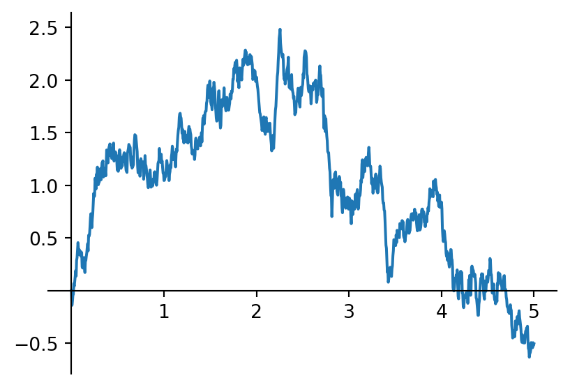
Brownian motion has many very interesting and well studied properties, a few of which we’ll discuss in the rest of this section. As it is always good to have a visual for what a “typical” path looks like, see Figure Figure 8.1.

Figure 8.1: A “typical” path $t \mapsto B_t(\omega)$ of a Brownian motion for $t \in [0,5]$, cf. Definition 8.2

Remark 8.2. Observe how the path in Figure 8.1 is continuous yet very spiky/jittery (in line with the description of the phenomenoms it was designed to model). In fact, this spiky/jittery behaviour remains present no matter how much you zoom in i.e. if you take a (typical) path, pick an arbitrary small time interval and zoom in on that interval it still shows that same spiky/jittery behaviour (so fractal like).

Here is an interesting way to construct a Brownian motion (for simplicity on a finite time interval $[0,1]$). Fix some (small) $h>0$ with $N=1/h$ integer. Consider on the time interval $[0,1]$ the grid consisting of time points $t_k=nh$ for $n=0,1,\ldots,N$. Define on these grid points the random walk (recall from Example 5.3 e.g.) $(X_n)_{n=0,1,\ldots,N}$ given by \[X_0=0 \quad \text{and} \quad X_n=\sum_{i=1}^n Y_i \quad \text{for all } n=1,2,\ldots,N,\] where the $Y_i$’s are independent copies of a random variable $Y$ taking values $\pm \sqrt{h}$ with probability $1/2$ each.

Then by the Central Limit Theorem, $X_N$ (located at $t_N=1$) has in the limit for $h \downarrow 0$ a $\mathcal{N}(0,1)$ distribution (so as a Brownian motion has at time $t=1$). But in fact you can prove a much stronger result: if we consider this random walk as a continuous time process on the interval $[0,1]$, simply by keeping it constant in between the grid points (while ensuring the cadlag property, cf. Definition 8.1, i.e. for any $t \in (t_k,t_{k+1})$ set the process equal to its value in $t=t_k$), then this guy as a process converges to a Brownian motion on the time interval $[0,1]$ as $h \downarrow 0$. This result is known as Donsker’s theorem (obviously, as we haven’t discussed what convergence of processes exactly means we don’t have the tools to make this more precise).

With some visual imagination this construction links the plot we made in Figure 5.2 (b) of a path of a simple random walk, after proper rescaling, to that of a path of a Brownian motion as in Figure 8.1. It also underlines the above “zooming in” comment: fixing any time interval $[t_1,t_2]$, no matter how small, the random walk approximation above shows that for (very) small $h$, also in this time interval the random walk will still see (very) many (small) up and downwards movements and hence the Brownian motion as its limit look very spiky/jittery.

Exercises

You can now do Exercise 8.2–Exercise 8.3.

8.3.1 Local path behaviour

Of course the paths of Brownian motion are quite intriguing with that fractal like, spiky behaviour discussed in Remark 8.2, and an interesting question is whether we can specify its properties a bit more precisely. Here are some results in that direction.

We start by introducing the concept of total variation of a function (which we’ll in moment apply to the paths of Brownian motion):

Definition 8.3 Let $f:[a,b] \to \R$ be a function. A grid $\Pi$ on $[a,b]$ is a collection of points, \[\Pi=\{t_0,\ldots,t_n\}, \tag{8.6}\] so that $a=t_0<t_1<\ldots<t_n=b$, and the corresponding grid size $\lvert \Pi \rvert$ is the maximal distance between its elements: \[\lvert \Pi \rvert :=\max_{k=1,\ldots,n} (t_k-t_{k-1}).\]

For a grid $\Pi$ as in Equation 8.6 we define the variation of $f$ over $\Pi$ as \[V_\Pi(f) := \sum_{k=1}^n \lvert f(t_k)-f(t_{k-1}) \rvert. \tag{8.7}\] Then the total variation of $f$ is defined as \[V(f) := \sup_{\Pi} V_\Pi(f) \in [0,\infty] \tag{8.8}\] where the supremum is taken over all possible grids (for any number of points $n=2,3,\ldots$).

We say that $f$ has/is of bounded variation if $V(f)<\infty$ and unbounded variation otherwise. Note that we can equivalently formulate this as follows: $f$ is of bounded variation if and only if there exists a (finite) constant $C>0$ so that $V_\Pi(f) \leq C$ for any possible grid $\Pi$.

Finally consider the special case that $f:[a,b] \to \R$ is continuous. Let $\Pi_1, \Pi_2, \ldots$ be any sequence of grids so that $\lvert \Pi_m \rvert \to 0$ as $m \to \infty$. Then \[V(f) = \lim_{n \to \infty} V_{\Pi_m}(f). \tag{8.9}\] Sometimes Equation 8.9 is more convenient to work with than the general definition Equation 8.8, in particular because it allows you to choose a sequence of grids which can be quite handy. (I can’t seem to find a reference for this result in the books I have on my desk — it’s not too hard to prove using uniform continuity of $f$ though, if you’re keen then have a look here e.g.)

A nice and natural interpretation of $V(f)$ is as follows: if you walk along the graph of $f$, then $V(f)$ equals the total length you travel along the vertical axis as you do so. For example, consider the functions $f_{1,2}: [0,1] \to \R$ given by \[f_1(x)=x \quad \text{and} \quad f_2(x)=\begin{cases} 2x & \text{if $x \in [0,1/2]$} \\ 2-2x & \text{if $x \in (1/2,1]$.} \end{cases} \] Walking along the graph of $f_1$ you walk from the origin to the point $(1,1)$ i.e. you travel a distance of $1$ along the vertical axis so $V(f_1)=1$. For the graph of $f_2$, you first walk from the origin to $(1/2,1)$ i.e. a distance along the vertical axis of $1$, and then from $(1/2,1)$ to $(1,0)$ adding another distance of $1$ along the vertical axis, so that in total $V(f_2)=2$. To see these values from the definition, for $f_1$ see Exercise 8.4 (part i) and for $f_2$, relying on Equation 8.9, just take any sequence of grids $\Pi_1, \Pi_2, \ldots$ so that each of them contains the point $1/2$. You can then easily compute, using the monotonicity of $f_2$ on the intervals $[0,1/2]$ and $(1/2,1]$, that $V_{\Pi_m}(f)=2$ for all $m=1,2,\ldots$.

Now, clearly if you follow the graph of a very jittery/spiky/rough function, then you move up and down the vertical axis a lot, resulting in a large total variation. So in this sense the total variation is a natural measure for how jittery/spiky/rough a function is. In Exercise 8.4 we discuss some examples to get some more feel for total variation, and in particular when it is finite and when it is infinite.

As I’ve been trying hard so far to impress on you just how jittery/spiky/rough a (typical) path of a Brownian motion is, the following result won’t come as too much of a surprise:

Proposition 8.1 Consider a Brownian motion $(B_t)_{t \geq 0}$ on some probability space $(\Omega,\mathcal{F},\P)$. Fix any two time points $0 \leq T_1<T_2$. Then almost surely, a path $t \mapsto B_t(\omega)$ is of unbounded variation on the time interval $[T_1,T_2]$.

Note that the point of introducing the interval $[T_1,T_2]$ is just to stress that a typical path of Brownian motion is of unbounded variation on any time interval in $[0,\infty)$!

Proof. For any $\omega \in \Omega$, consider the path $t \mapsto B_t(\omega)$ for $t \in [T_1,T_2]$ and denote by $V(\omega)$ its total variation on that interval. In this way, $V: \Omega \to [0,\infty]$ is a random variable (with $\infty$ as possible value), and the statement of the proposition that we need to prove reads as \[\P \left( V=\infty \right) =1. \tag{8.10}\]

Let’s first introduce some ingredients that we will need. For any $n=1,2,\ldots$, consider the equidistant grid $\Pi_n=\{t_0, \ldots,t_n\}$ on the time interval $[T_1,T_2]$ consisting of the points $t_k=T_1+k(T_2-T_1)/n$ for all $k=0,\ldots,n$, and let $V_{\Pi_n}(\omega)$ be the variation of the path $t \mapsto B_t(\omega)$ over this grid i.e. (cf. Equation 8.7) \[V_{\Pi_n}(\omega)=\sum_{k=1}^n \lvert B_{t_k}(\omega)-B_{t_{k-1}}(\omega) \rvert. \tag{8.11}\] Observe that since $V(\omega)$ is the total variation of the path $t \mapsto B_t(\omega)$ we have that (cf. Equation 8.8) \[V(\omega) \geq V_{\Pi_n}(\omega) \quad \text{for all } n=1,2,\ldots \text{ and all } \omega \in \Omega. \tag{8.12}\] Further note that, like $V$, $V_{\Pi_n}: \Omega \to [0,\infty)$ is a random variable.

Now, we can break the proof up in the following steps.

For any $M=1,2,\ldots$ fixed we have that \[\lim_{n \to \infty} \P \left( V_{\Pi_n} \leq M \right)=0.\]
For any $M=1,2,\ldots$ fixed we have that \[\P(V \leq M)=0.\]
It holds that $\P(V=\infty)=1$.

Step 1. Fix some $M=1,2,\ldots$. Note that Equation 8.11 shows that $V_{\Pi_n}$ is the sum of the absolute values of $n$ increments of $(B_t)_{t \geq 0}$, which by Definition 8.2 iii are independent random variables, and by Definition 8.2 iv (and the fact that we have chosen an equidistant grid) they all have the same distribution: the absolute value of a $\mathcal{N}(0,(T_2-T_1)/n)$ distributed random variable. This guy is actually pretty well known as the folded Normal distribution, see e.g. Wiki. In particular we have expressions for its mean and variance: \[\E[\lvert B_{t_k}-B_{t_{k-1}} \rvert]=\frac{c_1}{\sqrt{n}} \quad \text{and} \quad \var(\lvert B_{t_k}-B_{t_{k-1}} \rvert)=\frac{c_2}{n},\] where for simplicity/brevity we set the constants \[c_1=\sqrt{\frac{2(T_2-T_1)}{\pi}} \quad \text{and} \quad c_2=(T_2-T_1) \left( 1-\frac{2}{\pi} \right).\] Using linearity of expectation and variance (due to independence) it follows from Equation 8.11 that \[\E[V_{\Pi_n}]=n \frac{c_1}{\sqrt{n}} = c_1 \sqrt{n} \quad \text{and} \quad \var(V_{\Pi_n})=n \frac{c_2}{n}=c_2. \tag{8.13}\] Here we also see the key insight behind the whole proof really: as $n$ grows, $\E[V_{\Pi_n}]$ grows to $\infty$ while $\var(V_{\Pi_n})$ remains constant. So the larger $n$ becomes, for $V_{\Pi_n}$ to take a value smaller than the fixed $M$ that value needs to be an ever increasing multiple of $\var(V_{\Pi_n})$ below $\E[V_{\Pi_n}]$. We know that the probability that this happens becomes ever smaller, and a tool like Chebyshev’s inequality allows us to make this rigorous.

Indeed we can for instance argue as follows, for any $n$ large enough so that $\E[V_{\Pi_n}]=c_1 \sqrt{n}>M$: \[\begin{align*} \P(V_{\Pi_n} \leq M) &= \P \big( V_{\Pi_n}-\E[V_{\Pi_n}] \leq M-\E[V_{\Pi_n}] \big) \\ &\leq \P \big( \lvert V_{\Pi_n}-\E[V_{\Pi_n}] \rvert \geq \E[V_{\Pi_n}]-M \big) \\ &\leq \frac{1}{\E[V_{\Pi_n}]-M} \E \big[ \lvert V_{\Pi_n}-\E[V_{\Pi_n}] \rvert \big] \\ &\leq \frac{1}{\E[V_{\Pi_n}]-M} \left( 1+\var(V_{\Pi_n}) \right) \\ &\leq \frac{1+c_2}{c_1 \sqrt{n}-M}, \end{align*} \] so that by taking the limit we indeed arrive at \[\lim_{n \to \infty} \P \left( V_{\Pi_n} \leq M \right) \leq \lim_{n \to \infty} \frac{1+c_2}{c_1 \sqrt{n}-M}=0.\] We have used the following in the above. On the second line (which probably looks more complicated than it actually is) we used that for some random variable $X$ and constant $a<0$: \[\lvert X \rvert \geq -a \iff X \leq a \text{ or } X \geq -a,\] so in terms of events $\{ X \leq a \} \subseteq \{ \lvert X \rvert \geq -a \}$. The third line uses Chebyshev’s inequality (cf. Proposition 3.6 v) where the role of the non-negative random variable $X$ is played by $\lvert V_{\Pi_n}-\E[V_{\Pi_n}] \rvert$ and the role of the positive constant $a$ by $\E[V_{\Pi_n}]-M$. The fourth line uses that since $\lvert x \rvert \leq 1+x^2$ for all $x \in \R$, we have that \[\E \big[ \lvert V_{\Pi_n}-\E[V_{\Pi_n}] \rvert \big] \leq 1+\E \left[ \big( V_{\Pi_n}-\E[V_{\Pi_n}] \big)^2 \right]\] and further we just plugged in the definition of variance. The final line then simply plugs in the values for the expectation and variance from Equation 8.13.

Steps 2&3: cf. Exercise 8.5.

Another property that screams “rough paths!” is the following. It’s not very surprising having seen Proposition 8.1 and Exercise 8.4 ii. If you’re interested in a proof, see e.g. exercise 2.9 in Revuz and Yor (1993).

Proposition 8.2 Almost surely, a path of Brownian motion is nowhere differentiable. That is, if $(B_t)_{t \geq 0}$ is a Brownian motion on some probability space $(\Omega,\mathcal{F},\P)$, then the event consisting of all $\omega \in \Omega$ for which the path $t \mapsto B_t(\omega)$ is differentiable at some $t \in [0,\infty)$ has probability $0$.

Exercises

You can now do Exercise 8.4–Exercise 8.5.

8.3.2 Scaling and transformations

Next let’s look at the (remarkable) fact that you can apply certain transformations to a Brownian motion to create new processes that are themselves also Brownian motions!

Proposition 8.3 Let $(B_t)_{t \geq 0}$ be a Brownian motion on some probability space $(\Omega,\mathcal{F},\P)$. Then the following four processes $(B^{(i)}_t)_{t \geq 0}$, each defined as a transformation of $(B_t)_{t \geq 0}$, are also Brownian motions on this space:

$B^{(1)}_t=-B_t$ for all $t \geq 0$ (symmetry),
for any constant $c>0$ fixed, $B^{(2)}_t=cB_{t/c^2}$ for all $t \geq 0$ (scale invariance),
$B^{(3)}_0=0$ and $B^{(3)}_t=t B_{1/t}$ for all $t > 0$ (time inversion),
for any $T \geq 0$ fixed, $B^{(4)}_t=B_{T+t}-B_T$ for all $t \geq 0$ (time homogeneity).

Proof. Obviously we need to check that each of the four processes satisfy the properties from Definition 8.2. Recall that in general, if $Z\sim \mathcal{N}(\mu,\sigma^2)$ then for any constants $a,b \in \R$ \[aZ+b \sim \mathcal{N}(a\mu+b,a^2 \sigma^2). \tag{8.14}\]

For the first one this is all pretty clear: the independence in part iii of Definition 8.2 is obviously preserved if you multiply evertything by $-1$, and for part iv of Definition 8.2 an increment $B^{(1)}_{t_2}-B^{(1)}_{t_1}=-(B_{t_2}-B_{t_1})$ still has a $\mathcal{N}(0,t_2-t_1)$ distribution (cf. Equation 8.14).

Similarly for the second one and the fourth one. For the second one, note that an increment \[B^{(2)}_{t_2}-B^{(2)}_{t_1}=c(B_{t_2/c^2}-B_{t_1/c^2})\] is equal in distribution to $cZ$, where $Z \sim \mathcal{N}(0,(t_2-t_1)/c^2)$, which using Equation 8.14 again amounts to a $\mathcal{N}(0,t_2-t_1)$ distribution.

The third one is probably a bit less obvious (this is partly due to our choice of how to formulate Definition 8.2). The most elegant/easiest way to approach it is via properties of Gaussian processes, of which Brownian motion is a particular example. We don’t really want to spend time on that in this course, but see e.g. Proposition 1.10 in Revuz and Yor (1993) if you are interested. Note that continuity of its paths is obvious for $t \in (0,\infty)$ but it is less obvious what happens if $t \downarrow 0$. Note that (just make the substitution $s=1/t$) \[\lim_{t \downarrow 0} B^{(3)}_t = \lim_{t \downarrow 0} t B_{1/t} = \lim_{s \to \infty} \frac{B_s}{s}\] and hence a.s. continuity of paths holds provided that \[\lim_{s \to \infty} \frac{B_s}{s}=0 \quad \text{(a.s.).} \tag{8.15}\] Observe that if we focus on integers $n=1,2,\ldots$ then we can write a.s. \[\lim_{n \to \infty} \frac{B_n}{n} = \lim_{n \to \infty} \frac{1}{n} \sum_{k=1}^n (B_k-B_{k-1}), \tag{8.16}\] simply using that $B_0$ a.s. (property i in Definition 8.2) and a telescoping series. Now, these increments $B_k-B_{k-1}$ appearing in this sum are mutually independent and have a common $\mathcal{N}(0,1)$ distribution (properties iii & iv in Definition 8.2), so that it follows from the Strong Law of Large Numbers that Equation 8.16 equals $0$ a.s. This helps, but is not entirely giving us Equation 8.15 just yet: for that we also need to control what happens at the time points in between the integers. This could be done independently using Kolmogorov’s inequality and the Borel–Cantelli lemma e.g. (but obviously don’t worry about this for exam purposes).

One thing we can learn from Proposition 8.3 is that Brownian motion is not a unique process (in any sense): even on the same probability space, if a Brownian motion exists then each of the transformations in Proposition 8.3 creates a new, different process on that space which is also a Brownian motion. Besides that, Proposition 8.3 is very useful to study further properties of Brownian motion — we’ll see some of that in action in Proposition 8.4 below.

8.3.3 Long term behaviour

Next we briefly look at how Brownian motion tends to behave at larger time scales, in particular as $t \to \infty$. As a little bit of preparation, first the following. Recall that for some $T>0$ fixed, any continuous function $f:[0,T] \to \R$ is guaranteed to be bounded (both below and above) and it attains both its minimum/infimum and maximum/supremum⁷, this is just the classic extreme value theorem from elementary calculus.

⁷ If you’d like a reminder about sup/inf and how they compare to max/min, see e.g. Wiki

If we now consider a continuous function $f:[0,\infty) \to \R$ (like a typical path of Brownian motion) then when it comes to its largest value there are two possibilities:

$\sup_{t \geq 0} f(t)=s \in \R$ (i.e. the supremum has a finite value), then $f$ is bounded above by $s$ i.e. $f(t) \leq s$ for all $t \geq 0$; or
$\sup_{t \geq 0} f(t)=\infty$, then $f$ is not bounded above i.e. for any $a>0$ (no matter how large), there exists a $t \geq 0$ so that $f(t)>a$.

You can write down the analogue for its lowest value, making the distinction between $\inf_{t \geq 0} f(t) \in \R$ and $\inf_{t \geq 0} f(t) =-\infty$.

With that in our pocket, we will prove below that almost surely, a path $t \mapsto B_t(\omega)$ of a Brownian motion has the property that \[\sup_{t \geq 0} B_t(\omega)=\infty \quad \text{and} \quad \inf_{t \geq 0} B_t(\omega)=-\infty \tag{8.17}\] i.e. the path is neither bounded above by any positive nor bounded below by any negative level. It achieves this by acting somewhat like a sine function with ever increasing amplitude: as $t$ increases it keeps fluctuating between positive and negative values, gradually reaching ever higher and ever lower levels. Of course, crucially important here is that the time axis $[0,\infty)$ has infinite length to make such behaviour possible.

Now, the weaker statement that almost surely a path satisfies \[\sup_{t \geq 0} B_t(\omega)=\infty \quad \text{\emph{or}} \quad \inf_{t \geq 0} B_t(\omega)=-\infty \tag{8.18}\] is actually not very hard to see, via an argument we have used previously for random walks as well. Essentially, if a path does not satisfy Equation 8.18, then there exists an $a>0$ so that the path is bounded below by $-a$ and above by $a$ i.e. the whole path $t \mapsto B_t(\omega)$ is contained in the strip between $-a$ and $a$. But this is only possible if all increments of the path over the integers, i.e. \[B_1-B_0, B_2-B_1, \ldots\] are in absolute value no larger than $2a$ — as you can easily see, any increment with an absolute value larger than $2a$ necessarily makes the path escape the strip. And since these increments are independent of each other (cf. Definition 8.2 iii) and all have a $\mathcal{N}(0,1)$ distribution (cf. Definition 8.2 iv), by the “monkey typing Shakespeare” argument (recall from Section 7.3.1) the probability that all increments are in absolute value no larger than $2a$ is simply $0$. By taking the union over (e.g.) all integer $a=1,2,\ldots$, we capture all paths for which Equation 8.18 does not hold in one event, and this event then also has probability $0$ by the continuity property of (probability) measures (cf. Theorem 1.1 iv).

If you’re not entirely convinced yet about the difference between the weaker and stronger statement above, then consider for instance the trivial deterministic process $(X_t)_{t \geq 0}$ given by $X_t=t$. This satisfies Equation 8.18 (because $\sup_{t \geq 0} X_t = \sup_{t \geq 0} t=\infty$) but not Equation 8.17 (because $\inf_{t \geq 0} X_t = \inf_{t \geq 0} t=0$). Or, slightly more interesting example maybe: $(X_t)_{t \geq 0}$ given by $X_t=Y t$, where $Y$ is a random variable with possible values $-1$ and $1$.

Proposition 8.4 Let $(B_t)_{t \geq 0}$ be a Brownian motion on some probability space $(\Omega,\mathcal{F},\P)$. Then we have the following:

\[\P \left( \sup_{t \geq 0} B_t=\infty \text{ and } \inf_{t \geq 0} B_t =-\infty \right)=1, \tag{8.19}\]
Law of Large Numbers for Brownian motion: \[\P \left( \lim_{t \to \infty} \frac{B_t}{t}=0 \right)=1.\]

Proof. For property ii, that’s nice and easy: recall from Proposition 8.3 iii and the (sketch of the) proof of that proposition that this follows from path continuity (in particular in $t=0$) of the process defined in part iii of that proposition.

For property i, this takes a few steps, and is also a grand tour along almost all the transformations we have seen in Proposition 8.3! Define the random variable $Z: \Omega \to [0,\infty]$ by $Z(\omega):=\sup_{t \geq 0} B_t(\omega)$. To justify the codomain $[0,\infty]$, note that we indeed have that (cf. Definition 8.2 i) \[Z(\omega)=\sup_{t \geq 0} B_t(\omega) \geq B_0(\omega)=0\] and note that we include $\infty$ as possible value for $Z$.

We break the proof up in a number of steps:

For any $c>0$, $Z$ and $cZ$ have the same distribution.
For any $0<a<b<\infty$ we have that $\P(Z \in (a,b))=0$.
It holds that $\P(Z=0)+\P(Z=\infty)=1$.
It holds that $\P(Z=\infty)=1$.
The result, Equation 8.19, follows.

Step 1: fix any $c>0$. Recall from Proposition 8.3 ii that the process $(W_t)_{t \geq 0}$ given by $W_t=cB_{t/c^2}$ is also a Brownian motion, and hence $\sup_{t \geq 0} W_t$ has the same distribution as $\sup_{t \geq 0} B_t$ i.e. as $Z$ (see Remark 8.3 for a brief explanation of the justification). But we can easily work out that \[\sup_{t \geq 0} W_t = \sup_{t \geq 0} cB_{t/c^2} = c \sup_{t \geq 0} B_{t/c^2} = c \sup_{t \geq 0} B_{t} = cZ\] (the fourth equality just because $t/c^2$ runs through the whole interval $[0,\infty)$ just as $t$ itself does), i.e. $cZ$ has the same distribution as $Z$.

Step 2: fix any $0<a<b<\infty$, and let $\alpha:=\P(Z \in (a,b))$. Assume that $\alpha>0$, and we will derive a contradiction. Set $\beta:=b/a>1$ so that we can conveniently write \[(a,b)=(a,\beta a)=:I_0. \tag{8.20}\] The trick is now to use the result of step 1 to construct other intervals, all disjoint from $I_0$, where $Z$ also ends up with probability $\alpha$, leading to a probability of larger than $1$ and hence a contradiction. To execute this, for any $n=0,1,\ldots$ define the following constants and intervals: \[c_n=\beta^{-2n} \quad \text{and} \quad I_n=(a \beta^{2n},a\beta^{2n+1})\] (note that $I_0$ here is consistent with $I_0$ in Equation 8.20). Observe that the $I_n$’s form an increasing sequence of intervals in the sense that the left endpoint of $I_{n+1}$ is larger than the right endpoint of $I_n$: \[a \beta^{2(n+1)} = a \beta^{2n+2)} > a\beta^{2n+1}\] so in particular they are mutually disjoint. Further we have that \[\P(Z \in I_n) = \P(Z \in (a \beta^{2n},a\beta^{2n+1})) = \P(c_n Z \in (a,\beta a))= \P(Z \in (a,\beta a))=\alpha,\] where the second equality uses the def of $c_n$, the third that $c_n Z$ has the same distribution as $Z$ by step 1, and the final one the def of $\alpha$.

Now, since each $I_n \subseteq (0,\infty)$ we get by countable additivity (cf. Definition 1.3 — recall that the events below are mutually disjoint since the $I_n$’s are, cf. Lemma 2.1) that \[\P(Z \in (0,\infty)) \geq \sum_{n=0}^\infty \P(Z \in I_n) = \sum_{n=0}^\infty \alpha = \infty,\] the final step by our assumption that $\alpha>0$. Obviously this conclusion is contradicting the fact that $\P(Z \in (0,\infty)) \leq \P(\Omega)= 1$.

Step 3: note that we can write the event $\{ Z \in (0,\infty)\}$ as a union of an increasing sequence of events: \[\{ Z \in (0,\infty) \}=\bigcup_{n=1}^\infty \{ Z \in (1/n,n) \},\] so that by continuity of $\P$ (cf. Theorem 1.1 iv) and step 2 we get that \[\P(Z \in (0,\infty))=\lim_{n \to \infty} \P(Z \in (1/n,n)) = \lim_{n \to \infty} 0=0.\] Since for any $\omega \in \Omega$, $Z(\omega) \in [0,\infty]$ as mentioned at the start of the proof, we have that $\P(Z \in [0,\infty])=1$, and since obviously \[\{ Z \in [0,\infty] \} = \{Z=0\} \cup \{ Z \in (0,\infty) \} \cup \{Z=\infty\},\] the result follows by taking probabilities and countable additivity (cf. Definition 1.3).

Step 4: we will show that $\P(Z=0)=0$, so that the result follows from step 3. For this, from Proposition 8.3 iv with $T=1$ we know that the process $(W_t)_{t \geq 0}$ given by $W_t=B_{t+1}-B_1$ is yet another Brownian motion and hence \[\sup_{t \geq 0} W_t = \sup_{t \geq 0} (B_{t+1}-B_1)=\sup_{t \geq 0} B_{t+1}-B_1\] has the same distribution as $Z$. Note that for $\omega \in \Omega$ with $Z(\omega)=0$, we have that \[B_1(\omega) \leq \sup_{t \geq 0} B_t(\omega)=Z(\omega) =0\] as well as \[\sup_{t \geq 0} B_{t+1}(\omega)-B_1(\omega) \leq Z(\omega)-B_1(\omega)=-B_1(\omega)<\infty.\] In terms of events we can write this as \[\{ Z=0 \} \subseteq \{ B_1 \leq 0 \} \cap \left\{ \sup_{t \geq 0} B_{t+1}-B_1<\infty \right\}\] and taking probabilities it follows that \[\begin{align*} \P(Z=0) &\leq \P \left( B_1 \leq 0 \ \& \ \sup_{t \geq 0} B_{t+1}-B_1<\infty \right) \\ &= \P \left( B_1 \leq 0 \ \& \ \sup_{t \geq 0} B_{t+1}-B_1=0 \right) \\ &= \P(B_1=0) \P \left( \sup_{t \geq 0} B_{t+1}-B_1=0 \right) \\ &= \frac{1}{2} \P(Z=0), \end{align*} \tag{8.21}\] where the second and last line use that $\sup_{t \geq 0} B_{t+1}-B_1$ has the same distribution as $Z$ and hence in particular is a.s. either $0$ or $\infty$ by step 3, the third that any increment $B_{t+1}-B_1$ is independent of $B_1$ (cf. Definition 8.2 iii), and the last line also uses that $B_1 \sim \mathcal{N}(0,1)$ (cf. Definition 8.2 iv).

Finally, the ultimate left and right hand side of Equation 8.21 reads as $\P(Z=0) \leq \P(Z=0)/2$. Clearly this fails to hold if $\P(Z=0)>0$, so it must be true that $\P(Z=0)=0$.

Step 5: I wouldn’t want you to miss out on all the fun ;) so we’ll leave this one for you to do in Exercise 8.6.

We immediately get the following interesting consequence pretty much for free:

Corollary 8.1 If $(B_t)_{t \geq 0}$ is a Brownian motion on some probability space $(\Omega,\mathcal{F},\P)$, then almost surely a path will hit/visit any level $a \in \R$ infinitely often. That is, with $\#A$ denoting the number of elements a set $A$ contains, we have for any $a \in \R$ that \[\P \big( \# \{ t \in [0,\infty) \, | \, B_t=a \}=\infty)=1.\]

Proof. Fix some $a \in \R$ and suppose that a (continuous) path $t \mapsto B_t(\omega)$ hits/visits it only finitely often. Pick some $T>0$ larger than the last time $a$ is hit/visited, so that for all $t \in (T,\infty)$ we have either $B_t(\omega)<a$ or $B_t(\omega)>a$. We claim that in the former case we have that $\sup_{t \geq 0} B_t(\omega)<\infty$ while in the latter case we have that $\inf_{t \geq 0} B_t(\omega)>-\infty$, so that it follows from Proposition 8.4 that indeed such a path has probability $0$ only.

To see the claim, say that $B_t(\omega)<a$ for all $t>T$. On the time interval $[0,T]$, since the path is continuous it has a finite maximum (recall e.g. the extreme value theorem), say $b$. So $\sup_{t \geq 0} B_t(\omega)$ is bounded above by $\max\{a,b\}<\infty$. Analogue for the other case.

We conclude our intro to Brownian motion with two remarks.

Remark 8.3. (TL;DR for exam purposes below) as we have seen in Proposition 8.3, if on a certain probability space a Brownian motion exists then there exist many other processes that are also Brownian motions — in the sense that if $(B_t)_{t \geq 0}$ is a Brownian motion, then e.g. the process $(X_t)_{t \geq 0}$ given by $X_t=-B_t$ for all $t \geq 0$ is also a Brownian motion despite the fact that for any $\omega \in \Omega$, the paths $t \mapsto B_t(\omega)$ and $t \mapsto X_t(\omega)=-B_t(\omega)$ are not the same at all.

That also means that if we look at random variables defined as path functionals, such as the supremum, infimum and limit that all appear in Proposition 8.4, that these are not necessarily the same random variables for different Brownian motions. E.g. it will be the case that for (almost) any $\omega \in \Omega$, \[\sup_{t \geq 0} B_t(\omega) \not= \sup_{t \geq 0} -B_t(\omega).\] Nevertheless we have used in the proof of Proposition 8.3 several times that these suprema have the same distribution. How do we exactly justify that?

Now, in general it is of course well possible that two different random variables i.e. different mappings $\Omega \to \R$ have the same distribution, recall e.g. Example 2.3. But it is not at all clear from Definition 8.2 that any two processes satisfying the conditions in that def should have path functionals with the same distribution right?

Without going into too much detail, the justification relies on the following. Any Brownian motion necessarily has the same finite dimensional distributions (fdds) — recall that we briefly mentioned these guys in Remark 8.1. Writing $\Q_{> 0}$ for the non-negative rationals i.e. $\Q_{> 0} := \Q \cap (0,\infty)$ (countable!), it follows via continuity of $\P$ that if $(B_t)_{t \geq 0}$ and $(X_t)_{t \geq 0}$ are both Brownian motions and $\{A_q\}_{q \in \Q_{> 0}}$ a sequence of Borel sets then we have that \[\P \left( \bigcap_{q \in \Q_{> 0}} \{ B_q \in A_q \} \right) = \P \left( \bigcap_{q \in \Q_{> 0}} \{ X_q \in A_q \} \right).\] This implies for instance that the random variables \[\sup_{q \in \Q_{> 0}} B_q \quad \text{and} \quad \sup_{q \in \Q_{> 0}} X_q\] have the same distribution. By continuity, the supremum over $q \in \Q_{> 0}$ is equal to the supremum over $t \in [0,\infty)$ (cf. Exercise 8.1) and so it follows that \[\sup_{t \geq 0} B_t \quad \text{and} \quad \sup_{t \geq 0} X_t\] have the same distribution as well.

TL;DR (don’t worry about the above for exam purposes): any path functional (determined by the values a path takes on the non-negative rationals) will have the same distribution for any Brownian motion.

Remark 8.4. A natural (non-examinable!) question that arises from the results in Proposition 8.4 is at what “rate” a Brownian motion tends to grow as $t \to \infty$, i.e. can we identify a function $\varphi(t)$ so that $B_t/\varphi(t)$ tends to a non-zero (random) constant as $t \to \infty$? We see from Proposition 8.4 i that a constant function $\varphi$ doesn’t work, it will need to be something that is actually increasing in $t$. On the other hand, Proposition 8.4 ii shows that it must increase slower than the identity mapping $t \mapsto t$ does. It turns out that such a $\varphi$ does (pretty much) indeed exist and there is even a nice explicit expression for it: \[\varphi(t)=\sqrt{2t \log(\log(1/t))}.\] This result is known as the Law of the Iterated Logarithm, see e.g. Theorem 1.9 in Revuz and Yor (1993) if you’re interested.

Exercises

You can now do Exercise 8.6.

8.4 Poisson processes

Finally in this chapter we would like to introduce the Poisson process. On the one hand this process shares some important properties with Brownian motion, on the other hand its paths look very different and contrary to Brownian motion, this process is quite easy to construct and also easier to understand!

Like Brownian motion, this process has a clear ‘real world’ motivation, namely as a counting process. Imagine counting the (seemingly) random number of occurences of some phenomenom over time, like particles getting emitted from some radioactive material, or you experiencing another delay while waiting for the bus to campus, or Kevin the Dog desperately needing a treat, etc. For any time $t \geq 0$, let $N_t$ denote the number of occurences that happened in the time interval $[0,t]$. Then we should clearly have

$N_0=0$,
for any time $t>0$, $N_t \in \{0,1,\ldots\}$,
for any $0 \leq t \leq s$, $N_s \geq N_t$.

The Poisson process is the most basic model within this class of counting processes, that comes about under some additional assumptions on how the occurences behave. Let’s start with the definition⁸.

⁸ If you look into other sources you may well encounter seemingly different definitions of a Poisson process. However they are ultimately all (mostly) interchangeable, and the exact formulation is motivated by the angle of discussion. In our case, we come from a Lévy process angle as will become clearer later on

Definition 8.4 A process $(N_t)_{t \geq 0}$ on some probability space $(\Omega,\mathcal{F},\P)$ is called a Poisson process with intensity $\lambda>0$ if it has the following properties:

$N_0=0$ (a.s.),
Each path $t \mapsto N_t(\omega)$ is cadlag,
For any $0 \leq t_1<t_2$, the increment $N_{t_2}-N_{t_1}$ is independent of the collection $\{ N_s \, | \, s \in [0,t_1]\}$,
For any $0 \leq t_1<t_2$, the increment $N_{t_2}-N_{t_1}$ has a $\text{Poisson}(\lambda (t_2-t_1))$ distribution.

Some notes:

Recall that we discussed the cadlag property of functions/paths in Equation 8.4 & Equation 8.5: in brief it means that the path is right-continuous resp. has a left limit at any $t \in [0,\infty)$ resp. $t \in (0,\infty)$.
Recall that a Poisson distributed random variable has range $\{0,1,2,\ldots\}$, so it follows from properties i and iv (and Exercise 2.9) that $N_t \sim \text{Poisson}(\lambda t)$ has range $\{0,1,2,\ldots\}$.
Note that the intensity $\lambda>0$ is a parameter for this process which plays a role in property iv.

Note how many similarities there are in this definition with the one for Brownian motion (cf. Definition 8.2): both a Poisson process and a Brownian motion start from $0$ at time $t=0$ and have independent (property iii) and stationary (property iv) increments. A stark difference (besides continuous vs cadlag paths) is in the distribution at any fixed time $t > 0$: Poisson vs Normal. The class of all processes that have stationary, independent increments, to which both Brownian motion and the Poisson process belong, are known as Lévy processes and we’ll look at this class as a whole in more detail in Chapter 10.

We promised above that constructing a Poisson process is nice and easy, so let’s do that next. Once we’ve done that we also know what a (typical) path of a Poisson process looks like and can talk a bit more about its properties.

Exercises

You can now do Exercise 8.7.

8.4.1 Construction of a Poisson process

Consider a probability space $(\Omega,\mathcal{F},\P)$ on which an i.i.d. (independent and identically distributed) sequence of random variables $H_1, H_2, \ldots$ lives, with a common $\text{Exp}(\lambda)$ distribution (recall its properties from Wiki) for some $\lambda>0$. Based on these we define another sequence of random variables $J_0, J_1, \ldots$ as the partial sums of the $H_i$’s: \[J_0=0, \quad J_1=H_1, \quad J_2=H_1+H_2, \quad \ldots\] i.e. \[J_0=0, \quad J_k=\sum_{i=1}^k H_i \quad \text{for all } k=1,2,\ldots \tag{8.22}\] (don’t feel confused: $J_0=0$ just means that $J_0$ is a trivial constant random variable).

Recall that at the start of Section 8.4 we talked about the motivation being wanting to count occurences of some phenomenom over time. We interpret $0<J_1<J_2<\ldots$ as the (random) time points at which we observe the first, second, … occurence of the phenomenom. We call these the arrival times. Observe that for any $k=1,2,\ldots$ we have that \[J_k-J_{k-1}=\sum_{i=1}^k H_i - \sum_{i=1}^{k-1} H_i=H_k, \tag{8.23}\] i.e. $H_k$ is the amount of time we have to wait after the $k-1$-th occurence until we observe the next, the $k$-th occurence. Therefore we call $H_1, H_2, \ldots$ the interarrival times. Note that we have introduced $J_0=0$ as an auxiliary time just to be able to write down Equation 8.27 also for $k=1$, other than $J_1, J_2, \ldots$ it does not actually signal an occurence arriving.

Recall also that we said that we want our process to count the number of occurences over time. That is, for any $t \geq 0$ we set \[N_t = \text{the number of occurences in the time interval } [0,t] \in \{0,1,\ldots \} \tag{8.24}\] i.e. $N_t$ equals the number of time points $J_1, J_2, \ldots$ that satisfy $J_k \leq t$: \[N_t = \#\{ J_k \, | \, k \geq 1 \ \& \ J_k \leq t \} \tag{8.25}\] (where $\#A$ is notation for the number of elements in a set $A$).

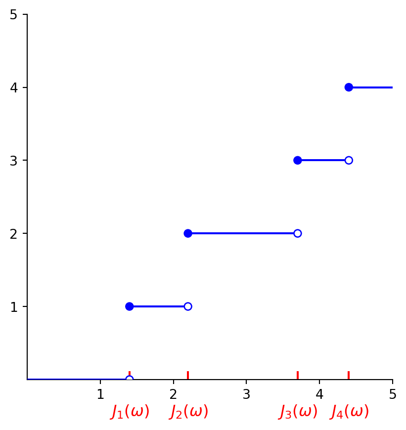
The above is the perspective of the random variable $N_t$ at some fixed time point $t \in [0,\infty)$. Alternatively we could equivalently also consider what happens if we fix an $\omega \in \Omega$ so that the occurences happen at the time points $0<J_1(\omega)<J_2(\omega)<\ldots$ (no longer random!) and we let time $t$ run to understand what the corresponding path $t \mapsto N_t(\omega)$ looks like. Think about sitting there with a piece of paper and pen, pressing “start” on your mobile phone to let the timer start, and at any time $t \geq 0$ let $N_t(\omega)$ be the number of occurences you have observed. You start at level $0$ at time $t=0$ and keep $N_t(\omega)$ constant at level $0$ until we get to time $t=J_1(\omega)$ when you observe the first occurence and you increase $N_t(\omega)$ from $0$ to $1$. Next you keep $N_t(\omega)$ constant at level $1$ until we get to $t=J_2(\omega)$ when you observe the second occurence and increase $N_t(\omega)$ from $1$ to $2$. Etc. for all eternity (I know!). In a formula this looks as follows: \[N_t(\omega)=\begin{cases} 0 & \text{if $t \in [0,J_1(\omega))$} \\ 1 & \text{if $t \in [J_1(\omega),J_2(\omega))$} \\ 2 & \text{if $t \in [J_2(\omega),J_3(\omega))$} \\ \vdots & \quad \vdots \end{cases} = \sum_{k=0}^\infty k \mathbf{1}_{\{ t \in [J_{k-1}(\omega),J_k(\omega)) \}} \tag{8.26}\] (note that the latter expression, using a sum of indicator functions, is in the same spirit as we’ve used these before: for any $\omega \in \Omega$ and any $t \in [0,\infty)$, only one term in the summation is not zero).

Note that the path/function $t \mapsto N_t(\omega)$ described by Equation 8.26 is a piecewise constant one: it has a jump upwards of size $1$ whenever we cross one of the $J_k(\omega)$’s and that’s all the movement we get out of it. Also note that we have chosen the setup so that the path is cadlag (cf. Equation 8.4 & Equation 8.5): for any $k=1,2,\ldots$ we have that $N_{J_k(\omega)}(\omega)=k$ and also $N_{J_k(\omega)+h}(\omega)=k$ for all $h>0$ small enough (so that $J_k(\omega)+h<J_{k+1}(\omega)$), ensuring right-continuity.

Some minor technical details to iron out: in order for the above to work as we want, we do need to have that for any $\omega \in \Omega$ \[0=J_0(\omega)<J_1(\omega)<J_2(\omega)<\ldots \tag{8.27}\] as well as \[\lim_{k \to \infty} J_k(\omega) = \lim_{k \to \infty} \sum_{i=1}^k H_i(\omega)=\infty. \tag{8.28}\] I appreciate that it may not be obvious but our key assumption that the $H_i$’s are i.i.d. with common $\text{Exp}(\lambda)$ distribution actually does not guarantee that these conditions hold⁹, nevertheless the good news is that they can fail to hold on an event of probability $0$ only and that we can then simply create a new probability space by excluding the $\omega$ in that event without hurting any aspects of our construction.

⁹ If a random variable $X$ has an $\text{Exp}(\lambda)$ distribution then this does not guarantee that $X(\omega)>0$ for all $\omega \in \Omega$, only that $\P(X>0)=1$ (cf. Exercise 2.9 e.g.). Also it is not impossible that $\lim_{k \to \infty} J_k(\omega)$ is actually finite, but this requires that $\lim_{k \to \infty} H_k(\omega)=0$ and due to the independence of the $H_k$’s, by a variation of the “monkey typing Shakespeare” argument this happens with probability $0$ only

Here is the confirmation that this construction works:

Lemma 8.1 We have the following.

On a probability space $(\Omega,\mathcal{F},\P)$, let $H_1, H_2, \ldots$ be an i.i.d. (independent and identically distributed) sequence of random variables with a common $\text{Exp}(\lambda)$ distribution, for some $\lambda>0$. Define the sequence of random variables $J_0, J_1, \ldots$ as in Equation 8.22. We can assume without loss of generality that Equation 8.27 and Equation 8.28 hold.

Then the process $(N_t)_{t \geq 0}$ given by one/all of Equation 8.24, Equation 8.25, Equation 8.26 is a Poisson process with intensity $\lambda$ as defined in Definition 8.4.
The converse is also true: if $(N_t)_{t \geq 0}$ is a Poisson process on a probability space $(\Omega,\mathcal{F},\P)$, then $(N_t)_{t \geq 0}$ has the structure as discussed in this section, where the random variables $J_1, J_2, \ldots$ and $H_1, H_2, \ldots$ can be deduced from the jumps in the paths of $(N_t)_{t \geq 0}$.

Further, we call the $J_1, J_2, \ldots$ the arrival times and the $H_1, H_2, \ldots$ the interarrival times of the process.

Finally, recalling from your basic probability courses that a sum of i.i.d. Exponentially distributed random variables has a Gamma distribution (see e.g. Wiki), it follows from Equation 8.22 that for any $k=1,2,\ldots$ \[J_k \sim \text{Gamma}(k,\lambda).\] Be aware that there are two distinct parametrisations of the Gamma distribution in common use — we use the “shape/rate” parametrisation rather than the “shape/scale” one.

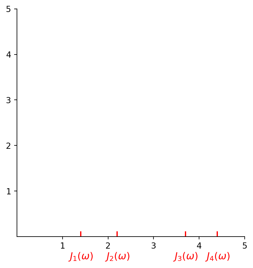
See Figure 8.2 below for a visualisation of what a path of a Poisson process (based on this construction) looks like. Have a good stare at it and convince yourself that it indeed aligns with the above construction!

For the sake of saving some time/amount of material, we won’t go into a detailed proof of this result, if you’re interested then see e.g. Section 6.8 in Grimmett and Stirzaker (1992). However, note that properties i and ii in Definition 8.4 are clearly satisfied by our construction. Property iii, that an increment $N_{t_2}-N_{t_1}$ is independent of what happened up until (incl.) time $t_1$, well the only real problem there is with the arrival of the first occurence after time $t_1$, this will influence the value of $N_{t_2}-N_{t_1}$ but since we already started waiting for that occurence before time $t_1$ it seems to create a dependency on what happened before time $t_1$ — in particular, how long we are already waiting for it at time $t_1$ would normally affect how much longer we still have to wait after time $t_1$. However this is where the choice for an Exponential distribution for the interarrival times pays off: its lack of memory property ensures that, in fact, there is no such dependence! For a proof that $N_t$ as constructed in this section indeed has a $\text{Poisson}(\lambda t)$ distribution, as property iv (together with property i) in Definition 8.4 requires, see Exercise 8.8.

(a) The arrival times on the time axis, in this case $J_1(\omega)=1.4$, $J_2(\omega)=2.2$, $J_3(\omega)=3.7$ and $J_4(\omega)=4.4$ — of course there’s $J_5(\omega), J_6(\omega), \ldots$ as well but these are all larger than $5$ in this case so don’t show up in the visual. Observe that the corresponding interarrival times (e.g. using Equation 8.27) equal $H_1(\omega)=1.4$, $H_2(\omega)=0.8$, $H_3(\omega)=1.5$ and $H_4(\omega)=0.7$

Exercises

You can now do Exercise 8.8.

8.4.2 Some properties of Poisson processes

We conclude this chapter with a brief discussion of some properties of Poisson processes, in particular also to compare & contrast with Brownian motion. We already mentioned that, at least superficially, their definitions (cf. Definition 8.2 & Definition 8.4) share quite some similarities. But then, if you compare what their typical paths look like they could hardly be any different (cf. Figure 8.1 & Figure 8.2)!

Indeed where a (typical) path of Brownian motion is continuous, of unbounded variation on any time interval (cf. Proposition 8.1) and reaching arbitrarily high&low levels (cf. Proposition 8.4), a path of a Poisson process is not continuous (still cadlag though), non-decreasing and therefore of bounded variation on any time interval $[0,T]$ (cf. Exercise 8.4 i) and reaches arbitrarily high values (but not negative ones).

Further it is good to point out that Poisson processes come with a parameter, its intensity $\lambda>0$. Hence it is rather actually a whole family of processes. Recall from Section 8.4.1 above that $\lambda$ feeds as parameter into the common Exponential distribution that the interarrival times $H_1, H_2, \ldots$ share. Recall that its mean is $1/\lambda$, i.e. for small values of $\lambda$ its mean is quite large, implying that the waiting time between occurences/jumps of the Poisson process tends to be quite large (low intensity if you will). On the other hand, for large values $\lambda$ these waiting times tend to be quite short (high intensity).

Interestingly, if you consider the sum of two independent Poisson processes then you again get a Poisson process, see Exercise 8.9.

Finally, the fact that we have chosen an Exponential distribution for the interarrival times has some profound implications — indeed it is responsible for the fact that the resulting process has the stationary, independent increments property as briefly discussed in Section 8.4.1. Nevertheless it is interesting to consider what the process would look like if we had chosen a different distribution, or even different distributions depending on how many occurences we have already seen. For instance, even Kevin the dog will wait longer to ask for yet another treat if it has been a treatful day so far! This brings us to a class of stochastic processes called renewal processes — beyond the scope of this course, but if you’re interested see e.g. Section 8.3 in Grimmett and Stirzaker (1992).

Exercises

You can now do Exercise 8.9.

8.5 Some exercises

About the exercises

Each exercise has a (rough) indication of its difficulty, as follows:

*	easier: can be solved by (almost) only using relevant definitions/results,
**	medium: in addition to relevant definitions/results, needs a limited amount of work/creativity,
*******	harder: in addition to relevant definitions/results, needs a larger amount of work/serious creativity,
💀	warning: might make your brain hurt! These are mainly intended to provide some extra challenge for those of you keen on that and are generally quite hard. You don't need to worry about these too much for exam purposes.

The exam consists of mostly ** and *** level questions, some *, and possibly at most a few marks worth of 💀.

A bit of preaching: it is an incredibly important part of the study process to try and work on the exercises as much as possible. To become a better mathematician/learn new maths (and also to get a good exam mark ;)), above all you need to do it. And yes, of course that includes falling over things, and making mistakes, and getting stuck, and getting frustrated — all part of the game and what you’re supposed to be doing! Your lecturers have done that as well and still do it. What matters is that you don’t let that discourage you and that you make good use of the help and resources available to help you develop your skills. As part of that, many exercises have a hint in a block like this:

Hint (click to view)

Hint!

These are trying to help you on your way if you don’t know where to start or to provide some ideas if you get stuck. In spirit of the above, always have a look at these first and try again before you look at the full solution. (These hints are an extra service that won’t be available in the exam I’m afraid ;).)

Of course, we have our classes and there’s office hours, email etc. as well — I’m at any time very happy to help you with any questions you may have, and you should please never feel that any question is “too dumb” to ask!

Full/detailed solutions for the exercises will become available, just immediately below the exercises, after our Friday tutorial.

Exercise 8.1 [**] Suppose that $f: [0,\infty) \to \R$ is a right-continuous function. Show that the following two statements are equivalent:

$f(x)=0$ for all $x \in [0,\infty)$,
$f(x)=0$ for all non-negative rational $x$ i.e. for all $x \in \Q \cap [0,\infty)$.

Note that this also means, for instance, that if $f$ and $g$ are both right-continuous functions so that $f(x)=g(x)$ for all $x \in \Q \cap [0,\infty)$ then simply $f=g$ (just apply the above to the right-continuous function $f-g$). The general principle in words: a right-continuous function on the (uncountable!) set $[0,\infty)$ is fully determined by its values on the (countable!) set $\Q \cap [0,\infty)$.

Hint (click to view)

You’ll hopefully agree that i $\Rightarrow$ ii is trivial, and that the challenge is in showing that ii $\Rightarrow$ i. For this, the key is to combine right-continuity of $f$ with the fact that $\Q$ is dense in $\R$ (recall e.g. the brief discussion in Proposition 1.2 iv) and hence that the non-negative rationals $\Q \cap [0,\infty)$ are dense in $[0,\infty)$.

Full solution (click to view)

Since $\Q \cap [0,\infty)$ is a subset of $[0,\infty)$, it is obvious that i implies ii. Indeed the bit of work is in showing that ii implies i. Assume that ii holds and fix any $x \in [0,\infty)$. If $x$ is rational, then we get $f(x)=0$ immediately from ii. If $x$ is irrational (i.e. not in $\Q$), then because $\Q$ is dense in $\R$ (see e.g. the brief discussion in Proposition 1.2 iv) there exists a sequence $q_1, q_2, \ldots$ in $\Q$ so that $q_n \downarrow x$ as $n \to \infty$. By right-continuity of $f$, we have that \[f(x)=\lim_{n \to \infty} f(q_n).\] But since $q_n \in \Q$ we know from ii that $f(q_n)=0$ for all $n=1,2,\ldots$. So indeed it follows that \[f(x)=\lim_{n \to \infty} f(q_n)=\lim_{n \to \infty} 0=0.\]

Exercise 8.2 [*/**] On some probability space $(\Omega,\mathcal{F},\P)$, let $Z$ be a random variable with a $\mathcal{N}(0,1)$ distribution. Consider the stochastic process $(X_t)_{t \geq 0}$ given by $X_t= Z \sqrt{t}$ (so just the product of $Z$ with $\sqrt{t}$) for all $t \geq 0$. Is $(X_t)_{t \geq 0}$ a Brownian motion?

Hint (click to view)

We’ll need to verify whether or not the process $(X_t)_{t \geq 0}$ has the properties listed in Definition 8.2. If you start from the top, you should pretty quickly (and without too much hassle) run into one that fails to hold!

Full solution (click to view)

Well we’ll just need to check the properties of Definition 8.2 right. It is clear that $X_0=0$ and that for any $\omega \in \Omega$, $t \mapsto X_t(\omega)=Z(\omega) t$ is continuous. However property iii clearly fails: for any $0<t_1<t_2$, the increment $X_{t_2}-X_{t_1}=Z(\sqrt{t_2}-\sqrt{t_1})$ is not independent of the collection $\{ X_s \ | \, s \in [0,t_1] \}$ — in fact quite the opposite: for any $s \in [0,t_1]$, $X_s=Z \sqrt{s}$ and $X_{t_2}-X_{t_1}=Z(\sqrt{t_2}-\sqrt{t_1})$ are “fully dependent” on each other in the sense if you know the value of one of the two, you can compute the value of the other. Or, equivalently: we can express each one as a deterministic function of the other.

Note: observe that this process does have the property (shared with Brownian motion, see the final bullet point in Definition 8.2) that $X_t \sim \mathcal{N}(0,t)$ for all $t>0$. Further, looking at property iv in Definition 8.2, an increment $X_{t_2}-X_{t_1}=Z(\sqrt{t_2}-\sqrt{t_1})$ does have a Normal distribution with mean $0$, but its variance fails to be equal to $t_2-t_1$.

Exercise 8.3 [**] Let $(B_t)_{t \geq 0}$ be a Brownian motion on some probability space $(\Omega,\mathcal{F},\P)$. Show that for any $t,s \geq 0$ we have that $\cov(B_t,B_s)=\min\{t,s\}$.

Note: recall that for any two random variables $U,V$, their covariance is given by \[\cov(U,V)=\E \big[ (U-\E[U])(V-\E[V]) \big]=\E[UV]-\E[U]\E[V].\]

Hint (click to view)

Maybe you find it easiest to first consider the case $0 \leq t \leq s$ and then later the case $0 \leq s \leq t$. Obviously, make optimal use of the properties we know from Definition 8.2!

If you get stuck with a term $\E[B_t B_s]$, then here is a very useful trick: Definition 8.2 gives us a lot of info about increments of the process, so try to rewrite $B_t B_s$ (just with some algebra I mean!) to bring in an(y) increment.

Still don’t see the increment trick??

Ok, how about writing $B_t B_s=B_t (B_s-B_t)+B_t^2$ for instance?

Full solution (click to view)

First suppose that $0 \leq t \leq s$. We have that \[\cov(B_t,B_s)=\E[B_t B_s]-\E[B_t]\E[B_s]=\E[B_t B_s],\] where we used that $\E[B_t]\E[B_s]=0$ as both these random variables have a Normal distribution with mean $0$ (recall from the final bullet point in Definition 8.2).

To deal with $\E[B_t B_s]$, Definition 8.2 doesn’t tell us anything about such a product of random variables. Rather Definition 8.2 specifies a number of properties, including the distribution, of any increment of $(B_t)_{t \geq 0}$. So let’s try to rewrite $B_t B_s$ so that we bring in an increment! One way is to write \[B_t B_s=B_t (B_s-B_t)+B_t^2.\] Indeed this allows us to compute \[\begin{align*} \E[B_t B_s] &= \E[B_t (B_s-B_t)]+\E[B_t^2] \\ &= \E[B_t] \E[B_s-B_t]+\E[B_t^2] \\ &= 0+t, \end{align*} \] where the second line uses that the increment $B_s-B_t$ is independent of the collection $\{ B_u \, | \, u \in [0,t] \}$ and hence in particular also of $B_t$ so that we can apply Proposition 3.6 viii (with $f$ and $g$ just the identity mappings); and the third line uses that both $B_t$ (see the final bullet point in Definition 8.2) and $B_s-B_t$ (cf. Definition 8.2 iv) have expectation $0$ while since $B_t \sim \mathcal{N}(0,t)$ (again, see the final bullet point in Definition 8.2) \[t=\var(B_t)=\E[B_t^2]-\big( \E[B_t] \big)^2=\E[B_t^2].\]

So, under the assumption that $0 \leq t \leq s$ we ultimately find that $\cov(B_t,B_s)=t$. Obviously we can interchange the roles of $t$ and $s$ here (or, otherwise, repeat the above computation) to see that $\cov(B_t,B_s)=s$ if $0 \leq s \leq t$. So we can indeed conclude that for any $t,s \geq 0$ we have that $\cov(B_t,B_s)=\min\{t,s\}$.

Exercise 8.4 [**] In this exercise we look at some functions $f:[0,1] \to \R$ and try to figure out whether they are of bounded or unbounded variation.

Suppose that $f$ is a monotone function, i.e. either non-decreasing or non-increasing. Compute $V(f)$.
Suppose that $f$ is continuous on $[0,1]$, differentiable on $(0,1)$, and that $f'$ is a bounded function (i.e. a finite constant $c>0$ exists so that $\lvert f'(x) \rvert \leq c$ for all $x \in (0,1)$). Show again that $V(f)<\infty$.

Hint: recall the mean value theorem.
Let $f(x)=\sin(1/x)$ for $x>0$ and $f(0)=0$. Show that $V(f)=\infty$.

Note/hint: the function in part iii is not continuous in $0$, but that is not what causes the unbounded variation. That is rather because, if you let $x$ decrease to $0$, it experiences an unlimited number of fluctuations between its minimal and maximal values $-1$ and $1$. To convince you maybe a bit better that it is not the lack of continuity that is the problem, consider for instance the function $f(x)=x^2 \sin(1/x^2)$ for $x \not= 0$ and $f(0)=0$. That one is continuous and differentiable everywhere (including in $x=0$). Nevertheless on $[0,1]$ (or any other domain containing $0$), we have that $V(f)=\infty$!

Note that this is not a contradiction with part ii: you can check that $f'(x)=2x \sin(1/x^2)-2 \cos(1/x^2)/x$ for $x \not= 0$ and $f'(0)=0$ (to see the latter, just work out the difference quotient), so $f'$ is not bounded on any interval containing $0$.

Hint (click to view)

Obviously this is all about using Definition 8.3.

For i, first take $f$ to be non-decreasing. For any grid $\Pi=\{t_0,\ldots,t_n\}$ on $[0,1]$, write down $V_\Pi(f)$ as defined in Definition 8.3. Now use that $f$ is non-decreasing to show that $V_\Pi(f)$ simplifies to $f(1)-f(0)$ and the result immediately follows!

For ii, similar to part i, again write down $V_\Pi(f)$ as defined in Definition 8.3 for any grid on $[0,1]$. See what happens if you apply the mean value theorem to each of the intervals $[t_{k-1},t_k]$ defined by your grid.

For iii, for which values of $x \in [0,1]$ does it hold that $f(x)=-1$, and for which $f(x)=1$? Consider building a sequence of grids by including ever more points where $f$ takes these extreme values.

Full solution (click to view)

For i, let $f$ be a non-decreasing function. Intuitively, if you walk along the graph of $f$, then you start at the point $(0,f(0))$ and end at the point $(1,f(1))$, and during the walk you only ever go up (or stay flat). So the distance travelled along the vertical axis should simply be $f(1)-f(0)$ no?

To do this rigorously, using Definition 8.3, let $\Pi=\{t_0,\ldots,t_n\}$ be any grid on $[0,1]$, and note that \[\begin{align*} V_\Pi(f) &= \sum_{k=1}^n \lvert f(t_k)-f(t_{k-1}) \rvert \\ &= \sum_{k=1}^n f(t_k)-f(t_{k-1}) \\ &= f(t_n)-f(t_0) \\ &=f(1)-f(0), \end{align*} \] where the big (well actually it’s not that big!) trick is in the second equality: since $f$ is non-decreasing, we have that $f(t_k) \geq f(t_{k-1})$ i.e. $f(t_k) - f(t_{k-1}) \geq 0$ and so we can simply drop the absolute values. The remaining summation is a nice example of a telescoping series: all terms in there except for $f(t_n)$ and $f(t_0)$ simply cancel against each other! If you don’t immediately see this, just write out the summation as \[f(t_1)-f(t_0)+f(t_2)-f(t_1)+f(t_3)-f(t_2)+\ldots+f(t_n)-f(t_{n-1})\] and see the cancellations happen in front of your eyes.

So $V_\Pi(f)=f(1)-f(0)$ no matter what $\Pi$ is, and hence trivially also \[V(f)=\sup_\Pi V_\Pi(f)=f(1)-f(0).\]

It works in exactly the same way if $f$ is non-increasing, except that we then find $V(f)=f(0)-f(1)$ rather.

For ii, take any grid $\Pi=\{t_0,\ldots,t_n\}$ on $[0,1]$ and let’s stare at \[V_\Pi(f) = \sum_{k=1}^n \lvert f(t_k)-f(t_{k-1}) \rvert. \tag{8.29}\] The idea is now that on any of the intervals $[t_{k-1},t_k]$, we can apply the mean value theorem to get that an $\alpha \in (t_{k-1},t_k)$ exists so that \[f(t_k)-f(t_{k-1})=f'(\alpha) (t_{k-1}-t_k).\] Taking absolute values on both sides yields \[\lvert f(t_k)-f(t_{k-1}) \rvert = \lvert f'(\alpha) \rvert \lvert t_k-t_{k-1} \rvert \leq c(t_k-t_{k-1}),\] where the inequality uses the assumption on $f'$ and that $t_{k-1}<t_k$. Plugging this back into Equation 8.29 we see that \[V_\Pi(f) \leq \sum_{k=1}^n c(t_k-t_{k-1}) = c \sum_{k=1}^n t_k-t_{k-1} = c, \tag{8.30}\] where the final step uses again the telescoping series observation from part i to simplify the summation to $1$. Since Equation 8.30 yields a finite and constant upperbound for any grid $\Pi$, it follows indeed that also \[V(f)=\sup_\Pi V_\Pi(f) \leq c<\infty.\]

For iii, observe that \[\frac{1}{\pi/2+2\pi m} \quad \text{for $m=1,2,\ldots$}\] is an infinite sequence of points in the interval $[0,1]$ for each of which $f$ has the value $1$, and \[\frac{1}{3\pi/2+2\pi m} \quad \text{for $m=1,2,\ldots$}\] is similarly an infinite sequence of points in the interval $[0,1]$ for each of which $f$ has the value $-1$. So if you include in your grid the points \[t_{k-1}=\frac{1}{3\pi/2+2\pi m} \quad \text{and} \quad t_k=\frac{1}{\pi/2+2\pi m}\] for some choice of $m=1,2,\ldots$ then $\lvert f(t_k)-f(t_{k-1}) \rvert=2$. So just choose a sequence of grids $\Pi_1, \Pi_2, \ldots$ in which you include increasingly many such pairs of points, then $V_{\Pi_n}(f)$ will be at least as large as $2$ times the number of such pairs of points and you can let it tend to $\infty$ as $n \to \infty$.

Exercise 8.5 [**/***] Complete steps 2 & 3 in the proof of Proposition 8.1. Both can be done in a few lines. Use the result from step 1 to prove step 2, and then step 3 using the result from step 2.

Hint (click to view)

For step 2, just make use of Equation 8.12.

For step 3, consider expressing the event $\{V=\infty\}$ in terms of the events $\{V>M\}$ and recall the continuity properties of $\P$ from Theorem 1.1 iv & v.

Full solution (click to view)

For step 2, we see from Equation 8.12 that for any $n=1,2,\ldots$, if $V(\omega) \leq M$ then also $V_{\Pi_n}(\omega) \leq M$. So \[\P(V \leq M) \leq \P(V_{\Pi_n} \leq M).\] Since this inequality holds for all $n=1,2,\ldots$, it remains true if we take the limit: \[\P(V \leq M) \leq \lim_{n \to \infty} \P \left( V_{\Pi_n} \leq M \right)=0,\] where the equality uses Step 1.

For step 3, note that for any $\omega \in \Omega$ we have that $V(\omega)=\infty$ if and only if $V(\omega)>M$ for all $M=1,2,\ldots$. In terms of events this reads as \[\{V=\infty\}=\bigcap_{M=1}^\infty \{ V>M \}.\] It follows from Theorem 1.1 v that \[\P \left( V=\infty \right) = \lim_{M \to \infty} \P(V > M) = \lim_{M \to \infty} 1 =1,\] where the second equality uses Step 2.

Exercise 8.6 [**/***] Complete step 5 in the proof of part i of Proposition 8.4.

Hint: make use of the symmetry property of Brownian motion, cf. Proposition 8.3 i.

Hint (click to view)

Recall that in steps 1–4 of the proof we have already established that \[\P \left( \sup_{t \geq 0} B_t=\infty \right)=1.\] First use Proposition 8.3 i to show that this implies that \[\P \left( \inf_{t \geq 0} B_t=-\infty \right)=1\] (for some algebra with sups and infs, recall e.g. Wiki) and then apply Exercise 2.5 to deduce that the statement in part i of Proposition 8.4 indeed holds.

Full solution (click to view)

Using the setting from Proposition 8.4, we have already established in steps 1–4 of the proof that \[\P \left( \sup_{t \geq 0} B_t=\infty \right)=1. \tag{8.31}\] From Proposition 8.3 i we know that the process $(-B_t)_{t \geq 0}$ is also a Brownian motion on this space, and hence Equation 8.31 applies to this process as well, yielding \[1=\P \left( \sup_{t \geq 0} -B_t=\infty \right)=\P \left( -\inf_{t \geq 0} B_t=\infty \right)=\P \left( \inf_{t \geq 0} B_t=-\infty \right)\] (see e.g. Wiki for the second step). So both $\{ \sup_{t \geq 0} B_t=\infty \}$ and $\{ \inf_{t \geq 0} B_t=-\infty \}$ are almost sure events, and then so is their intersection (cf. Exercise 2.5) i.e. \[\P \left( \sup_{t \geq 0} B_t=\infty \text{ and } \inf_{t \geq 0} B_t=-\infty \right)=1,\] and we’re done.

Exercise 8.7 [*/**] Let $(N_t)_{t \geq 0}$ be a Poisson process with intensity $\lambda>0$ that counts the number of treats that Kevin the dog eats. Time $t$ is measured in days.

What is the probability that Kevin eats no treats at all during a day?
Compute the probability that Kevin eats more than two treats during a three day period.
Compute the expected number of treats that Kevin eats during the first two days.
Compute the probability that Kevin eats 3 treats during the first two days, of which 2 during the first day.

Note: if needs be, recall the pmf and moments of a Poisson distribution from Wiki e.g.

Hint (click to view)

Parts i–iii can all be expressed as a probability/expectation of an increment of the process i.e. a random variable of the form $N_{t_2}-N_{t_1}$ for suitable choices of $0 \leq t_1<t_2$. Then it is a matter of using Definition 8.4 iv.

Part iv is of a slightly more complicated form, because if you write down the prob as described you end up with two (dependent) random variables you can’t do much with. However, exactly as in Exercise 8.3 (!), try to write it in terms of an increment because we do know how to deal with those — one of the similarities between Definition 8.4 and Definition 8.2!

Full solution (click to view)

A day is a time interval $[t,t+1]$ for some (integer) $t \geq 0$, and hence hence eating no treats means that $N_{t+1}-N_t=0$. From Definition 8.4 iv we get that $N_{t+1}-N_t \sim \text{Poisson}(\lambda)$ (that’s the stationary increments property in action: this distribution does not depend on what $t$ is i.e. which day we’re exactly looking at, only on the length of the time interval i.e. $1$ in this case) and hence the prob is (using the pmf of a Poisson distribution, using the above Wiki link or otherwise) \[\P(N_{t+1}-N_t=0)=e^{-\lambda}.\]
Analogue to part i, this translates to $N_{t+3}-N_t >2$ for some (integer) $t \geq 0$ and from Definition 8.4 iv we know that $N_{t+3}-N_t \sim \text{Poisson}(3 \lambda)$ so that we can compute \[\begin{align*} \P(N_{t+3}-N_t >2) &= 1-\P(N_{t+3}-N_t \leq 2) \\ &= 1- \big( \P(N_{t+3}-N_t =0)+\P(N_{t+3}-N_t =1)+\P(N_{t+3}-N_t =2) \big) \\ &= 1-e^{-3\lambda} \left( 1+3\lambda+\frac{9\lambda^2}{2} \right). \end{align*} \]
The number of treats eaten during the first two days is $N_2$, and from Definition 8.4 iv&i we know that $N_2=N_2-N_0 \sim \text{Poisson}(2 \lambda)$, so that $\E[N_2]=2\lambda$.
Note that we’re asked to compute $\P(N_1=2 \ \& \ N_2=3)$. This has the difficulty that it involves two dependent random variables and there’s seemingly not much we can do with this. However we’ve encountered a very similar situation before, indeed in Exercise 8.3, and the same idea used there can help us out here as well: rewrite/work towards an increment! Indeed we can write, using that Definition 8.4 iii guarantees that $N_2-N_1$ is independent of $N_1$ \[\P(N_1=2 \ \& \ N_2=3)=\P(N_1=2 \ \& \ N_2-N_1=1)=\P(N_1=2) \P(N_2-N_1=1),\] so that using (analogue to previous parts) $N_1=N_1-N_0 \sim \text{Poisson}(\lambda)$ and $N_2-N_1 \sim \text{Poisson}(\lambda)$ we arrive at \[\frac{\lambda^2}{2} e^{-\lambda} \cdot \lambda e^{-\lambda} = \frac{\lambda^3}{2} e^{-2 \lambda}.\]

Exercise 8.8 [**] In this exercise we will show that the Poisson distribution that pops up as part of the definition of a Poisson process indeed arises by choosing the interarrival times to be Exponentially distributed.

First we prove the following little help result. Show that for any $k=1,2,\ldots$, $\lambda>0$ and $t>0$ we have that \[\int_0^t \frac{\lambda^k}{(k-1)!} x^{k-1} e^{-\lambda x} \d x = 1-\sum_{j=0}^{k-1} \frac{(\lambda t)^j}{j!} e^{-\lambda t}. \tag{8.32}\]

Hint: consider using induction over $k$ and applying integration by parts.
Now consider a probability space $(\Omega,\mathcal{F},\P)$ on which a Poisson process $(N_t)_{t \geq 0}$ with intensity $\lambda>0$ lives. Prove, given that the interarrival times $H_1, H_2, \ldots$ are i.i.d. random variables with a common $\text{Exp}(\lambda)$ distribution and that $N_t$ is given by Equation 8.24 and/or Equation 8.25, that indeed $N_t \sim \text{Poisson}(\lambda t)$.

Hint: for any $k=1,2,\ldots$, consider expressing the event $\{N_t \geq k\}$ in terms of arrival times.

Hint (click to view)

For part i, if needs be refresh your memory on how induction works using the given Wiki link. Then, using integration by parts it is only a few lines of algebra!

For part ii, the key step is to argue that for any $k=1,2,\ldots$ we have the following relationship: $\{ N_t \geq k\}=\{J_k \leq t\}$. This allows to compute probabilities for $N_t$ using $J_k$, and recall that we do know what distribution the latter has (cf. Lemma 8.1). Together with part i that’s all you really need!

Full solution (click to view)

For part i, recall that a proof by induction consists of two steps:

Show that Equation 8.32 holds for $k=1$.
Assuming that Equation 8.32 holds for some $k=1,2,\ldots$, prove that it is then also true for $k+1$.

For step 1, plugging in $k=1$ you can easily work out that both sides of Equation 8.32 boil down to $1-e^{-\lambda t}$, so they are indeed equal.

For step 2, assume that Equation 8.32 holds for some $k=1,2,\ldots$ (induction hypothesis), and we’re looking to prove that \[\int_0^t \frac{\lambda^{k+1}}{k!} x^{k} e^{-\lambda x} \d x = 1-\sum_{j=0}^{k} \frac{(\lambda t)^j}{j!} e^{-\lambda t}. \tag{8.33}\] We can do this e.g. as follows: \[\begin{align*} \int_0^t \frac{\lambda^{k+1}}{k!} x^{k} e^{-\lambda x} \d x &= \left. \frac{\lambda^{k+1}}{k!} x^{k} \frac{-1}{\lambda} e^{-\lambda x} \right|_{x=0}^{x=t} - \int_0^t \frac{\lambda^{k+1}}{(k-1)!} x^{k-1} \frac{-1}{\lambda} e^{-\lambda x} \d x \\ &= -\frac{\lambda^k}{k!} t^k e^{-\lambda t} + \int_0^t \frac{\lambda^k}{(k-1)!} x^{k-1} e^{-\lambda x} \d x \\ &= -\frac{\lambda^k}{k!} t^k e^{-\lambda t} + 1-\sum_{j=0}^{k-1} \frac{(\lambda t)^j}{j!} e^{-\lambda t} \\ &= 1-\sum_{j=0}^{k} \frac{(\lambda t)^j}{j!} e^{-\lambda t} \end{align*} \] where the first line uses integration by parts and the third line uses the induction hypothesis.

For part ii, the key is to make the following connection: for any $k=1,2,\ldots$ fixed we have that $N_t(\omega) \geq k$ if and only if we have $k$ or more occurences in the interval $[0,t]$ i.e. if and only if the $k$-th occurence happens at or before time $t$ i.e. if and only if $J_k(\omega) \leq t$. In terms of events that means that we have $\{ N_t \geq k\}=\{J_k \leq t\}$, and hence \[\P(N_t \geq k)=\P(J_k \leq t)=\int_0^t \frac{\lambda^k}{(k-1)!} x^{k-1} e^{-\lambda x} \d x,\] where the second equality uses that $J_k \sim \text{Gamma}(k,\lambda)$ (cf. Lemma 8.1) and hence we can obtain the probability by integrating its pdf (recall from its formula from Wiki if needs be).

Now it follows from part i that we may also write \[\P(N_t \geq k)=1-\sum_{j=0}^{k-1} \frac{(\lambda t)^j}{j!} e^{-\lambda t}\] which yields \[\begin{align*} \P(N_t = k) &= \P(N_t \geq k)-\P(N_t \geq k+1) \\ &= 1-\sum_{j=0}^{k-1} \frac{(\lambda t)^j}{j!} e^{-\lambda t} - \left( 1-\sum_{j=0}^{k} \frac{(\lambda t)^j}{j!} e^{-\lambda t} \right) \\ &= \frac{(\lambda t)^k}{k!} e^{-\lambda t} \end{align*} \] which is exactly the pmf of a $\text{Poisson}(\lambda t)$ distribution!

Exercise 8.9 [**/***] On some probability space $(\Omega,\mathcal{F},\P)$, let $(N_t)_{t \geq 0}$ and $(M_t)_{t \geq 0}$ be independent Poisson processes with intensity $\lambda_N>0$ and $\lambda_M>0$ resp. Show that the sum of these two processes, i.e. the process $(Z_t)_{t \geq 0}$ given by $Z_t=N_t+M_t$ for all $t \geq 0$, is also a Poisson process. What is its intensity?

Hint: you may use that the sum of two cadlag functions is again a cadlag function (just to avoid the hassle of having to produce a fiddly proof for this) plus any facts you know about Poisson distributions.

Hint (click to view)

You hardly need to do any maths/algebra, it’s rather some reasoning to show that $(Z_t)_{t \geq 0}$ satisfies all the properties listed in Definition 8.4. If the “almost surely” in property i is causing you trouble, never forget about your loyal compaignon that is Exercise 2.5. For property iv, don’t forget about the basic properties of Poisson distributions, see e.g. Wiki.

Full solution (click to view)

We need to check that $(Z_t)_{t \geq 0}$ satisfies properties i–iv listed in Definition 8.4:

Observe that if $N_0(\omega)=0$ and $M_0(\omega)=0$, then also $Z_0(\omega)=N_0(\omega)+M_0(\omega)=0$. In terms of events we can write this as follows: \[\{ N_0=0\} \cap \{M_0=0\} \subseteq \{Z_0=0\}. \tag{8.34}\] Since $(N_t)_{t \geq 0}$ and $(M_t)_{t \geq 0}$ are both Poisson processes, we know both $\{ N_0=0\}$ and $\{ M_0=0\}$ are almost sure events. It follows from Exercise 2.5 that their intersection is also an almost sure event, and hence by Equation 8.34 (and Theorem 1.1 i) so is $\{ Z_0=0\}$.
Immediate from the hint.
Fix any $0 \leq t_1<t_2$. We can write the increment as \[Z_{t_2}-Z_{t_1}=N_{t_2}-N_{t_1}+M_{t_2}-M_{t_1}. \tag{8.35}\] Note that since $(N_t)_{t \geq 0}$ is a Poisson process, we know from Definition 8.4 iii that the increment $N_{t_2}-N_{t_1}$ is independent of the collection $\{N_s \, | \, s \in [0,t_1]\}$, and it’s also independent of the collection $\{M_s \, | \, s \in [0,t_1]\}$ since the processes are independent. Reasoning analogue for the increment $M_{t_2}-M_{t_1}$, it follows that $N_{t_2}-N_{t_1}$ and $M_{t_2}-M_{t_1}$ are both independent of the collection $\{M_s, N_s \, | \, s \in [0,t_1]\}$. Hence Equation 8.35 shows that $Z_{t_2}-Z_{t_1}$ is independent of the collection $\{M_s, N_s \, | \, s \in [0,t_1]\}$, and therefore also of the collection $\{Z_s \, | \, s \in [0,t_1]\}$.
Finally, again writing Equation 8.35, using that $N_{t_2}-N_{t_1} \sim \text{Poisson}(\lambda_N (t_2-t_1))$ and $M_{t_2}-M_{t_1} \sim \text{Poisson}(\lambda_M (t_2-t_1))$ and that they are independent, using the fact that the sum of independent Poisson distributed random variables is again Poisson distributed, with as parameter the sum of the parameters (see Wiki e.g.), it follows that $Z_{t_2}-Z_{t_1} \sim \text{Poisson}((\lambda_N+\lambda_M) (t_2-t_1))$.

We see from property iv above that $(Z_t)_{t \geq 0}$ has intensity $\lambda_N+\lambda_M$.

Note that this result is intuitively very nice: $(Z_t)_{t \geq 0}$ is formed by adding up the number of occurences from the source behind $(N_t)_{t \geq 0}$ and the source behind $(M_t)_{t \geq 0}$. The result tells us that (distribution wise at least) we may just as well look at the occurences from a third source, as long as the interarrival times from that third source have parameter $\lambda_N+\lambda_M$!