\[ \renewcommand{\P}{\mathop{\mathbb{P}}\nolimits} \newcommand{\E}{\mathop{\mathbb{E}}\nolimits} \newcommand{\var}{\mathop{\rm Var}\nolimits} \newcommand{\VaR}{\mathop{\rm VaR}\nolimits} \newcommand{\cte}{\mathop{\rm CTE}\nolimits} \newcommand{\cov}{\mathop{\rm Cov}\nolimits} \newcommand{\limsup}{\mathop{\rm limsup}} \newcommand{\liminf}{\mathop{\rm liminf}} \newcommand{\R}{\mathbb{R}} \newcommand{\Q}{\mathbb{Q}} \newcommand{\Z}{\mathbb{Z}} \newcommand{\N}{\mathbb{N}} \newcommand{\C}{\mathbb{C}} \renewcommand{\d}{\, \mathrm{d}} \newcommand{\dP}{\, \mathrm{d}\mathbb{P}} \newcommand{\eps}{\varepsilon} \renewcommand{\emptyset}{\varnothing} \]

7  Sharing and aggregating risks 1

7.1 Why?

After we saw some key ideas for quantifying risks as real numbers in Chapter 6, in the coming two chapters we’ll look at some more core activities for a risk manager responsible for a bunch of risks i.e. future random loss modelled by (non-negative) random variables: like pizzas and dogs and other things, you can share them with some other party, and you can aggregate them to look at a total risk/loss!

Risk sharing is (indeed) the concept of sharing/splitting up a risk \(X\) between multiple parties, according to some agreement. Basically trading in risks! Of course, no (rational) party will ever be keen to take on (partial) ownership, or increase their ownership share, of a risk without a (in their eyes) sufficient compensation in return. This compensation can take multiple forms, but most typically it is in the form of a payment when the agreement is signed (and where then the ideas around premium principles as discussed in Section 6.2 could play a role again!).

There are several steps involved and let’s write these down in a clear way, to make sure we’re on the same page:

Proposition 7.1 The process of sharing a risk \(X\) works as follows:

1. a sharing agreement is put in place, and possibly (premium) payments made from the party/ies that decrease their risk share to those that increase their risk share,
2. the risk \(X\) takes its value,
3. each party pays their part of that value, as dictated by the sharing agreement.

Here are some (of the many possible!) real world examples of risk sharing in action:

• Insurance. It is common for insurance policies to contain the concept of a deductible or an excess: if an event occurs causing damage that falls under the policy, then the insurance company pays out only part of that damage, the rest needs to be covered by the policyholder themselves. This is a form of risk sharing between the company and the policyholder: by entering into the insurance policy, the policyholder is no longer the sole owner of this risk but now shares it with the insurer. The cost of the policy is the price/premium the insurer requires to take ownership of part of this risk, and obviously how high the price/premium is depends on how the risk is shared exactly: the more risk for the insurance company (and the lesser for the policyholder), the higher the price/premium normally.

  Another form of risk sharing happens between insurance companies: if a company feels (or is told by a regulator) that it is too exposed to a certain category of risks, then it can offload some risk by sharing it with another insurance company. Obviously this is a business agreement, so they will have to pay a certain price/premium to that other company. Such arrangements go under the term reinsurance. There are a number of dedicated reinsurance companies (i.e. that only do business with other insurance companies) such as Axa Re, Swiss Re etc. In finance/banking and in several other industries similar arrangements occur.

• Joint ventures/partnerships. Companies regularly team up to set up a new piece of business/take on a (large) project together. This of course includes sharing the risks involved in some way. In this situation there may be some price/premium involved, but it can also be that all parties feel confident enough that their share of the profits will be high enough that they are all happy to take ownership of their part of the risk without further compensations between them.

• Securitisation etc. In corporate finance/banking, consumer debts like mortgages, car loans etc. are commonly bundled up and sold as a package to several buyers who then each (also) own part of the risk (so-called tranches) resulting from the danger that holders of such debts are not able to fulfil their financial obligations. In this case (as in the previous bullet point), this risk is accepted due to the prospect of the income stream they will receive (periodical payments made by the debt holders).

Risk aggregation is (indeed) adding multiple risks together to create a total/aggregate risk, say \(S\). In this part of the course we’ll generally be assuming that we’re dealing with independent risks/random variables — we discussed the (challenging!) complications that come with non-trivial dependenccy structures already in the copulas part of the course i.e. Chapter 3–Chapter 5. It may be that we are dealing with a given/known number of risks, say \(X_1, \ldots, X_n\) (random variables) for some given and fixed \(n\), so that \(S=X_1+\ldots+X_n\). Such sums you have seen before in earlier courses (see Section A.6 for a quick reminder of the key tools) and we don’t want to spend much time on those. Rather we’d like to focus on the more general and interesting situation that there may be some uncertainty around how many risks we’ll actually end up having to deal with/pay a non-zero amount for: the number of (actually relevant) risks is a random variable itself, say \(N\), and the total/aggregate risk is then \(S=X_1+\ldots+X_N\). Some real world examples where such a model naturally appears:

• Insurance. Imagine that you are working at an insurance company and are responsible for a portfolio (=collection) of insurance policies all of the same type (e.g. all car insurance policies) sold to policyholders with a similar risk profile. Under these assumptions, it makes sense to model the claim payments that you have to make to these policyholders, during say a year, as a sequence of i.i.d. (independent and identically distributed) sequence of random variables: \(X_1\) is the amount for the first claim payment, \(X_2\) is the amount for the second claim payment, etc. Obviously you wouldn’t know in advance how many of such payments you’re going to have to make, that depends on how car accidents e.g. that group of policyholders will experience during the coming year. So if we model this number as a random variable \(N\) with range (contained in) \(\{0,1,2,\ldots\}\), then your total outgo for this portfolio during a year is the random variable \(S=X_1+\ldots+X_N\).

• Operational risk. A project manager of say a large construction project has to take into account the risk of losses due to problems/failures with people, systems, equipment etc. Clearly the number of such losses, say \(N\), is uncertain and hence best modelled by random variable as in the previous example. The sizes of each of the losses are also random: \(X_1, \ldots, X_N\), so that the total/aggregate risk is again given by the random variable \(S=X_1+\ldots+X_N\).

  Note: for mathematical convenience we want to be working with i.i.d. random variables \(X_1, X_2, \ldots\). In this application, the independence is not too hard to justify, but the identical distribution property maybe less so: risks originating from different sources (people vs systems vs equipment vs …) may very well have different characteristics and hence needing different distributions no? A good way to deal with this in our modelling is to split the risks out in different categories and look at the aggregate risk/loss per category, say \(S_1, S_2, \ldots, S_k\). Then within each category the i.i.d. assumptions makes sense and we can use the tools we will discuss to analyse each of the \(S_i\)’s separately. And in the next chapter we will see a beautiful result allowing us to say useful things about the total aggregate risk/loss \(S_1+S_2+ \ldots +S_k\) we were actually after!

• Credit risk. Suppose that you’re an investor who has loaned money to a number of clients. In principle they will all pay you back, with a healthy portion of interest. But there is of course always the risk that some of them default i.e. that they can’t actually live up to their financial obligations, and that they can only repay you some part of the amount they owe you. If we let \(N\) denote the random number of clients that will default, and \(X_i\) the random amount you loose out on due to the \(i\)-th default, then your total risk/loss due to the defaults is given by \(S=X_1+\ldots+X_N\).

  We will look at credit risk in particular in more detail in the final two chapters!

7.2 Risk sharing

In Section 7.1 we discussed some real world occurences of risk sharing. Mathematically it means that a risk (i.e. non-negative random variable) \(X\) is shared between multiple parties i.e. is split up into \(n\) components (also non-negative random variables normally), say \(X_1, \ldots, X_n\), according to some rule/agreement. Rceall the process involved from Proposition 7.1. For convenience we’ll be focussing on the case \(n=2\) and we’ll write “\(Y\)” and “\(Z\)” rather than “\(X_1\)” and “\(X_2\)” resp. (that’s just because it’s more convenient notation later on) i.e. \[X=Y+Z. \tag{7.1}\]

The main question we wonder about is this: assuming that we know the distribution of the (total) risk \(X\), what is the distribution of each of the component risks \(Y\) and \(Z\)? If we can answer this, then the risk managers involved can go ahead and analyse the component they are responsible for (e.g., quantify using the techniques from Chapter 6) and, for instance, where relevant decide what price/premium they require to enter the risk sharing agreement.

Normally the sharing happens according to a particular rule set out in the agreement between the parties involved, i.e. functions \(f_1, f_2\) are specified so that \[Y=f_1(X) \quad \text{and} \quad Z=f_2(X).\] Obviously any such pair of functions should satisfy \[f_1(x)+f_2(x)=x \quad \text{for all } x \in \R, \tag{7.2}\] so that Equation 7.1 is guaranteed to hold: \[Y+Z=f_1(X)+f_2(X)=X.\]

Now, there is not so much in the way of useful general results here, the analysis happens mostly on a case-by-case basis. So let’s discuss some prominent examples of such agreements!

Remark 7.1. A few bits of advice to deal with the maths in this section.

Task I: Determining the distribution of \(Y\) and/or \(Z\). Generally you want to work with the cdf’s here (recall their def from Section A.1.1) of the random variables \(X, Y, Z\) rather than e.g. pdf’s, in particular because even if \(X\) is a continuous random variable and (hence) has a pdf then there is no guarantee at all that \(Y\) and \(Z\) are continuous random variables as well (generally this is only the case if both \(f_1\) and \(f_2\) is continuous and strictly monotone). Recall the brief discussion of “other” random variables in Section A.1.4.

Having established that, suppose that we know the cdf \(F_X\) of \(X\) and that we want to determine the cdf \(F_Y\) of \(Y=f_1(X)\) (the below story holds in the same way for the cdf \(F_Z\) of \(Z=f_2(X)\)). Then your natural first steps are to write \[F_{Y}(x)=\P(Y \leq x)=\P(f_1(X) \leq x) \quad \text{for all } x \in \R. \tag{7.3}\] But where do we go from here? Well in one of the following two directions.

1. In the special case that \(f_1\) is a one-to-one function, say that \(f_1\) is continuous and strictly increasing, and hence has a “classic” inverse \(f_1^{-1}\) (recall from Section 2.2.1!) we can further develop Equation 7.3 as \[\begin{align*} F_{Y}(x) &= \P(f_1(X) \leq x) \\ &= \P \left( f_1^{-1} \big( f_1(X) \big) \leq f_1^{-1}(x) \right) \\ &= \P \left( X \leq f_1^{-1}(x) \right) \\ &= F_X \left( f_1^{-1}(x) \right) \quad \text{for all } x \in \R, \end{align*} \tag{7.4}\] so in this case it is a matter of working out an expression for \(f_1^{-1}\), plugging that into \(F_X\) and all sorted!
2. Otherwise, if \(f_1\) is not one-to-one (or if you can’t find/don’t like using its inverse — this method always works!) then consider the following visual strategy if you can’t see an easier way (pun intended).
   1. Sketch the graph of \(f_1\).
   2. Let \(x\) run along the vertical axis in your sketch, from \(-\infty\)/bottom to \(\infty\)/top say, and for every \(x\) do the following:
      • find the set \(A\) of values on the horizontal (say \(w\)-)axis where the graph of \(f_1\) is less than or equal to \(x\) i.e. \[A=\{ w \in \R \, | \, f_1(w) \leq x \}\] so that \(w \in A \iff f_1(w) \leq x\);
      • then \(F_{Y}(x)=\P(f_1(X) \leq x)\) (cf. Equation 7.3) equals \(\P(X \in A)\) and we can (hopefully) work out \(\P(X \in A)\) using \(F_X\) (or whatever else we know about \(X\)).
   (You may hear some echoes here from Section 2.2.1: indeed this is nothing but a visual way of inverting \(f_1\) in a rather general sense!)

Task II: Determining expectations of \(Y\) and/or \(Z\). If rather than the whole distribution, you only need an expectation (of a function of) of \(Y\) and/or \(Z\) — such as the expectation itself, or a variance, or a higher moment, or a moment generating function etc. — then normally one of the well known Equation A.9 and Equation A.16 is all you need. For instance, if \(X\) is a continuous random variable with pdf \(f_X\) and we have a sharing agreement with \(Y=f_1(X)\), then \[\E[Y]=\E[f_1(X)]=\int_{-\infty}^\infty f_1(x) f_X(x) \d x = \ldots,\] \[\E \left[ Y^2 \right]=\E \left[ f_1(X)^2 \right]=\int_{-\infty}^\infty f_1(x)^2 f_X(x) \d x = \ldots,\] where the first one resp. the second one uses Equation A.16 with the choice \(h(x)=f_1(x)\) resp. \(h(x)=f_1(x)^2\). Etc.

7.2.1 Proportional sharing

The most straightforward form of risk sharing is simply proportional: each party is responsible for a certain percentage of the risk. That is, for some factor \(\alpha \in (0,1)\), called the retention level, we have that \[f_1(x)=\alpha x \quad \text{and} \quad f_2(x)=(1-\alpha)x\] or equivalently \[Y=\alpha X \quad \text{and} \quad Z=(1-\alpha) X.\] Mathematically this is not very complicated of course. For instance, to find the cdf \(F_Y\) of \(Y\) from the cdf \(F_X\) of \(X\) it is simply a matter of using their definitions and connecting them via a tiny bit of algebra: for any \(x \in \R\) \[\begin{align*} F_{Y}(x) &= \P(Y \leq x) \\ &= \P(\alpha X \leq x) \\ &= \P \left( X \leq \frac{x}{\alpha} \right) \\ &= F_X \left( \frac{x}{\alpha} \right) \end{align*} \tag{7.5}\] (nice to note: this is nothing but method 1 from Task I in Remark 7.1 in action, clearly \(f_1(x)=\alpha x\) is continuous and strictly increasing so one-to-one, with inverse \(f_1^{-1}(x)=x/\alpha\)).

Example 7.1 If the (total) risk \(X \sim \text{Exp}(\theta)\) for some \(\theta>0\) is shared proportionally with factor \(\alpha \in (0,1)\), i.e. \[Y=\alpha X \quad \text{and} \quad Z=(1-\alpha) X,\] then \(Y \sim \text{Exp}(\theta/\alpha)\) and \(Z \sim \text{Exp}(\theta/(1-\alpha))\).

To see this, recall that the cdf of an \(\text{Exp}(\theta)\) distributed random variable, say \(G\), is given by \[G(x)=\begin{cases} 1-e^{-\theta x} & \text{if } x>0 \\ 0 & \text{if } x \leq 0 \end{cases} \tag{7.6}\] (if you had forgotten, just deduce it from Equation A.12 using the pdf from Appendix B). Hence from Equation 7.5 and since \(F_X=G\) we readily get that the cdf \(F_Y\) of \(Y\) is given by \[\begin{align*} F_Y(x) &= F_X \left( \frac{x}{\alpha} \right) \\ &= G \left( \frac{x}{\alpha} \right) \\ &= \begin{cases} 1-e^{-\theta (x/\alpha)} & \text{if } x/\alpha >0 \\ 0 & \text{if } x/\alpha \leq 0 \end{cases} \\ &= \begin{cases} 1-e^{-(\theta/\alpha) x} & \text{if } x >0 \\ 0 & \text{if } x \leq 0. \end{cases} \end{align*} \] Comparing this with Equation 7.6, we see that \(Y\) has the cdf of an Exponential distribution, with parameter \(\theta/\alpha\). Since cdf’s uniquely determine distributions (recall from Section A.1.1), it indeed follows that \(Y \sim \text{Exp}(\theta/\alpha)\). You can do \(Z\) in exactly the same way of course.

Note that it’s merely a nice coincidence that \(Y\) and \(Z\) have the same type of distribution as \(X\), that’s generally not the case!

7.2.2 Excess of loss (or: stop-loss) sharing

Proportional sharing is simple and maybe the first sharing arrangement that comes to mind. But in terms of (extreme) risk reduction, it offers only limited benefit to either party involved: if \(X\) ends up taking a (very) large value, then, you know, a percentage of a (very) large value can still be (very) large! Other arragements exist that provide stronger protection to one of the parties. At the same time, obviously a party that seeks strong protection against a risk by means of a sharing agreement will have to pay a substantial enough amount/premium (in Step 1 of Proposition 7.1) to find interested parties!

A prominent example of this is excess of loss sharing, also known as stop-loss sharing. This works as follows. An amount \(K>0\) is specified in the agreement, (also) called the retention level. One of the parties (typically the original owner of the risk), called the cedant, is responsible for \(X\) up until the amount \(K\) only. The other party, the excess provider, is responsible (only) for the excess of \(X\) over \(K\). That is, the following is agreed:

• if \(X \leq K\), then the cedant pays the whole \(X\) and the excess provider pays nothing;
• if \(X>K\), then the cedant pays \(K\) and the excess provider pays the remainder i.e. \(X-K\).

A practical example of this is from insurance: typically a car insurance policy contains a deductible, say £500. Here the insurance company is the excess provider and the retention level is \(K=500\). If you accidentally scratch your car and the repair costs £150 i.e. we have \(X=150\), then you pay the whole £150 by yourself and the insurance company pays nothing. On the other hand, if you get involved in a serious accident and the repair costs say £800, so \(X=800\), then the you pay £500 (\(=K\)) and the insurance company pays the rest i.e. £300 (\(=X-K\)).

Clearly, if you own the risk \(X\) and are worried about its large possible values, then entering into such an excess of loss agreement, even though the excess provider will charge you a price/premium for it, can be an attractive option!

If we express this in maths and let \(Y\) resp. \(Z\) be the share of \(X\) for the cedant resp. for the excess provider, then we get \[Y = \begin{cases} X & \text{if } X \leq K \\ K & \text{if } X > K \end{cases} = \min\{X,K\}\] and \[Z = \begin{cases} 0 & \text{if } X \leq K \\ X-K & \text{if } X > K \end{cases} = \max\{X-K,0\}\] (convince yourself that this makes for a valid way of sharing i.e. that Equation 7.1 indeed holds). Or, equivalently of course, we could write \(Y=f_1(X)\) and \(Z=f_2(X)\) where the functions are given by \[f_1(x) = \begin{cases} x & \text{if } x \leq K \\ K & \text{if } x > K \end{cases} = \min\{x,K\} \tag{7.7}\] and \[f_2(x) = \begin{cases} 0 & \text{if } x \leq K \\ x-K & \text{if } x > K \end{cases} = \max\{x-K,0\}. \tag{7.8}\]

Example 7.2 Let (again) \(X \sim \text{Exp}(\theta)\) for some \(\theta>0\), and consider an excess of loss sharing agreement with retention level \(K>0\). Let’s see if we can figure out what the distribution of \(Y\) (the share of the cedant) and \(Z\) (the share of the excess provider) is! Recall from Equation 7.6 that the cdf of \(X\) is \[F_X(x)=\begin{cases} 1-e^{-\theta x} & \text{if } x>0 \\ 0 & \text{if } x \leq 0 \end{cases} \tag{7.9}\]

Clearly the situation is a bit less obvious here than it was in Example 7.1, so let’s be careful and follow the visual strategy from method 2 of Task I in Remark 7.1.

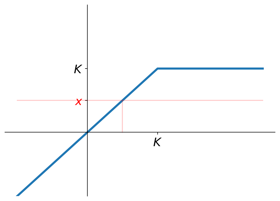
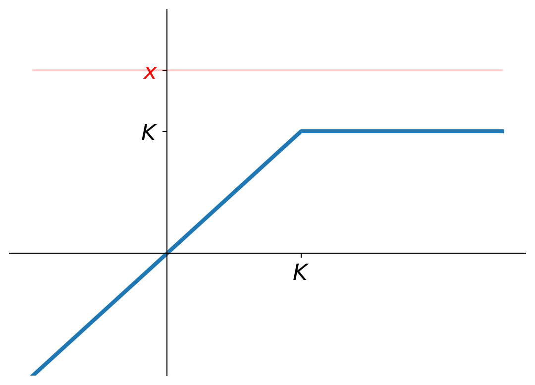
First for the cedant i.e. \(Y=f_1(X)\) with cdf \(F_Y\) to be determined, and where \(f_1\) is given by Equation 7.7. It is helpful that \(f_1\) is non-decreasing (it’s not one-to-one though!), making the analysis not too annoying. See Figure 7.1 for a plot of \(f_1\). Recall that we let \(x \in \R\) run over the vertical axis. We see that we should consider two cases:

1. Take \(x<K\). Cf. Figure 7.1 (a). Then we see that \(w\) (on the horizontal axis) satisfies \(f_1(w) \leq x\) if and only if \(w \leq x\) i.e. \(f_1(X) \leq x\) holds if and only if \(X \leq x\). Using this relationship (and otherwise all just by definition), we get that \[F_{Y}(x)=\P(Y \leq x)=\P(f_1(X) \leq x)=\P(X \leq x)=F_X(x). \tag{7.10}\]
2. Now take \(x \geq K\). Cf. Figure 7.1 (b). Now we see that any \(w\) (on the horizontal axis) satisfies \(f_1(w) \leq x\) (just because \(f_1(w) \leq K \leq x\)!). That is, no matter what value \(X\) takes, it is always true that \(f_1(X) \leq x\) holds and so this happens with probability \(1\): \[F_Y(x)=\P(Y \leq x)=\P(f_1(X) \leq x)=1. \tag{7.11}\] Note that this ties in perfectly with our understanding of this risk sharing agreement: the cedant never pays more than \(K\), and so the probability that \(Y\) is at most \(x\) is \(1\) for any \(x \geq K\)!

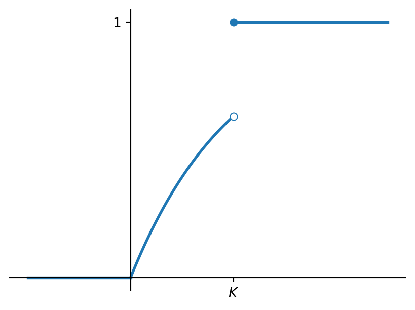
Combining Equation 7.10 and Equation 7.11, and recalling Equation 7.9, we arrive at the following expression for the cdf of \(Y\): \[F_Y(x)= \begin{cases} 0 & \text{if } x \leq 0 \\ 1-e^{-\theta x} & \text{if } x \in (0,K) \\ 1 & \text{if } x \geq K. \end{cases} \] For a plot of this guy, see Figure 7.2. Note that this plot shows that \(F_Y\) is neither a piecewise constant function nor a continuous function. Hence (cf. Section A.1.4) we have here an example of a situation we already warned for in Remark 7.1: even though \(X\) is a continuous random variable, \(Y\) is not a continuous random variable and neither a discrete random variable, it is an “other” one!

Next let’s do some moments of \(Y\). As mentioned in Task II in Remark 7.1, for this we can “just” go through Equation A.16 based on the relationship \(Y=f_1(X)\). And indeed that’s the only option we have here anyway: we have seen above that \(Y\) is neither a discrete nor a continuous random variable, so we can’t at all apply our knowledge for computing expectations from earlier Prob courses to this \(Y\) by itself!

Following the discussion in Task II in Remark 7.1, we have for instance for any \(k=1,2,\ldots\) that the first steps for working out the \(k\)-th moment \(\E[Y^k]\) look as follows: \[\begin{align*} \E[Y^k] &= \E \left[ f_1(X)^k \right] \\ &= \int_{-\infty}^\infty f_1(x)^k f_X(x) \d x, \end{align*} \] where \(f_X\) is the pdf of \(X\), and the second equality uses Equation A.16 with the choice \(h(x)=f_1(x)^k\). For the next steps, you plug in the expressions for \(f_X\) and for \(f_1\), and work stuff out.

For example, for \(k=1\) we get that \[\begin{align*} \E[Y] &= \E \left[ f_1(X) \right] \\ &= \int_{-\infty}^\infty f_1(x) f_X(x) \d x \\ &= \int_0^\infty \min\{x,K\} \theta e^{-\theta x} \d x \\ &= \int_0^K x \theta e^{-\theta x} \d x + \int_K^\infty K \theta e^{-\theta x} \d x \\ &= \frac{1}{\theta} - \left( K+\frac{1}{\theta} \right) e^{-\theta K} + K e^{-\theta K} \\ &= \frac{1}{\theta} \left( 1-e^{-\theta K} \right), \end{align*} \] where in the third equation we plug in the expressions for \(f_1\) and \(f_X\) (cf. Appendix B for the latter if you need a reminder), in the fourth we use that \(\min\{x,K\}\) is an annoying expression in an integral, so we use that \(\min\{x,K\}=x\) for all \(x \leq K\) and \(\min\{x,K\}=K\) for all \(x >K\) to break the integral up in two easier ones, and finally for the first integral in the fifth equality we use integration by parts (as also used in Example 6.1 e.g.).

Now you go analyse the situation for the excess provider, i.e. \(Z\), using the same ideas in Exercise 7.2!

(a) Considering \(x<K\)

(b) Considering \(x \geq K\)

Figure 7.1: A plot of \(f_1\)

Figure 7.2: A plot of \(F_Y\) (for \(\theta=1/2\) and \(K=2\))

7.3 Risk aggregation: compound distributions

Now we make the switch to the second topic in this chapter: risk aggregation. Recall that in Section 7.1 we already gave a brief introduction and some real world examples, which can generally be captured in the following framework:

• you as risk manager face a (possibly large) number of potential risks/losses: insurance policyholders that may submit a claim, operational risks that may materialise, debitors who may default on repaying their debts etc. We assume that these potential risks/losses do not influence each other (or at least not too much) and that they have an identical (or at least similar enough) profile in terms of the amount of money you stand to lose to them.
• you denote by \(N \in \{0,1,\ldots\}\) the number of these risks/losses that actually materialise (i.e. the other risk/losses end up not costing you anything);
• you denote by \(X_1, X_2, \ldots, X_N\) (all strictly positive) the sizes of the risks/losses that actually materialise (also called the severity of these risks/losses) — it doesn’t matter too much in which order you do that, maybe do it in order of time: \(X_1\) the size/severity of the very first risk/loss that turns out to materialise, \(X_2\) the second, etc.

then your total/aggregate risk/loss is given by the sum \[S=\sum_{i=1}^N X_i=X_1+\ldots+X_N. \tag{7.12}\] Obviously, rather than as an accouting tool for past events, we rather want to use this as a model for future events, say for the coming year. That means that we need to model all the uncertain ingredients as random variables:

• \(N\) as a random variable taking values in \(\{0,1,\ldots\}\) i.e. \(\text{Range}(N) \subseteq \{0,1,\ldots\}\), which makes it a so-called counting distribution, modelling the number of risks/losses that materialise in the coming year;
• \(X_1, X_2, \ldots\) a sequence of i.i.d. (independent and identically distributed) random variables that model the sizes/severities of the risks/losses that turn out to materialise. In our context/interpretation these will be strictly positive i.e. \(\text{Range}(X_i) \in (0,\infty)\), but for our mathematical analysis that aspect won’t matter a lot so it is not always assumed. Further, the reason that we take an infinite sequence here even though in Equation 7.12 we ever only need finitely many is merely a technical one that we will briefly discuss further below.

Under these assumptions, the random variable \(S\) that gives the total/aggregate risk/loss as expressed in Equation 7.12 is within Probability known as a so-called compound distrubution:

Definition 7.1 Suppose that:

• \(X_1, X_2, \ldots\) is a sequence of i.i.d. (independent and identically distributed) random variables,
• \(N\) is a random variable with range/set of possible values (contained in) \(\{0,1,\ldots\}\) (a so-called counting distribution), independent of \(X_1, X_2, \ldots\).

Then the distribution of the random variable \(S\) given by \[S=\sum_{i=1}^N X_i=X_1+\ldots+X_N, \tag{7.13}\] with the understanding that \(S=0\) if \(N=0\), is called a compound distribution.

Some notes:

• Note that Equation 7.13 is not properly defined if \(N=0\), therefore we explicitly add that we define \(S=0\) in that case. Of course that’s the natural thing to do: if \(S\) is the sum of no terms at all, then it should have the value \(0\) no, and in terms of aggregate risks/losses: if no risks/losses at all turn out to materialise, then you don’t have to pay anything.
• The more “classic” situation of a sum of \(n\) (fixed) i.i.d. random variables is a special case of a compound distribution: just let \(N\) be the trivial constant random variable \(N=n\).
• However, in general Equation 7.13 is (of course) a very different beast than your “classic” sum of a fixed number of i.i.d. random variables, and hence you cannot just apply any of the results you know for classic sums (the most important ones listed in Section A.6) to this \(S\) — instead we’ll have to build up some results for compound distributions from scratch!
• In our risk modelling application, we’ll normally want the \(X_i\)’s to be strictly positive random variables but this is not necessary as part of the general mathematical definition.
• Obvious I guess but just to have it pointed out: the fact that the \(X_i\)’s are identically distributed means that they all share the same “distributional properties” such as range, probablities/pdf/pmf, expectation/moments, generating functions etc. Therefore we typically use the word common when talking about any of these concepts for these random variables.

Just quickly about how this exactly works mathematically. Recall that random variables always live in the context of some experiment with outcome/sample space \(\Omega\), and that any random variable \(Z\) is a mapping/function from \(\Omega\) to \(\R\) (measuring some specific aspect about each possible outcome of the experiment). The thinking is: the experiment is done, an outcome \(\omega \in \Omega\) is observed, and then \(Z\) takes the value \(Z(\omega) \in \R\). Cf. Section A.1.

In this context, Equation 7.13 (just, exactly) means that the random variable \(S\) is defined as the mapping \(S: \Omega \to \R\) given \[S(\omega)=\sum_{i=1}^{N(\omega)} X_i(\omega) \in \R \quad \text{for all } \omega \in \Omega. \tag{7.14}\] So for any \(\omega \in \Omega\), each of the \(X_i\)’s in the above Definition 7.1 take a value on the real line: \(X_1(\omega) \in \R\), \(X_2(\omega) \in \R\), \(\ldots\), and \(N(\omega) \in \{0,1,\ldots\}\) (recall the condition on the range of \(N\) in the above Definition 7.1). The right hand side of Equation 7.14 is now “just” a “normal” sum of \(N(\omega)\) real numbers, giving a real number as value for \(S(\omega)\). In the special case that \(N(\omega)=0\), we understand \(S(\omega)=0\) (as mentioned in the above Definition 7.1).

So for any \(\omega \in \Omega\), only a finite number of the \(X_i(\omega)\)’s actually feed into the computation of \(S(\omega)\) via Equation 7.14, the other values (namely \(X_{N(\omega)+1}(\omega)\), \(X_{N(\omega)+2}(\omega)\), \(\ldots\)) are irrelevant. Why do we then insist on having an infinite number of them in Definition 7.1? This is just for purely technical reasons and has no further bearing/consequence/meaning: it ensures that we definitely have enough of them, no matter how large \(N(\omega)\) turns out to be, and it’s the clearest/cleanest way to formulate things mathematically since we want the \(X_i\)’s to be independent of \(N\).

Example 7.3 Suppose that you are managing two (identical) car insurance policies that we can assume to be independent of each other. Further we know the following for each policy: with probability \(1/4\) it generates a claim for you to pay, and if that happens then the claim amount can be modelled as an \(\text{Exp}(\theta)\) distribution, for some \(\theta>0\).

If we denote your aggregate risk/loss in this situation by \(S\) and use a compound distribution as in Definition 7.1 to express it, then:

• The number of risks/losses \(N\) i.e. claim payments that you’ll have to do in this situation has three possible values:
  • \(N=0\). This happens if neither policy generates a claim, i.e. with probability \(3/4 \cdot 3/4=9/16\).
  • \(N=1\). This means that you receive one claim in total, generated either by the first or by the second policy. The probability that this happens is hence \[\frac{1}{4} \cdot \frac{3}{4} + \frac{3}{4} \cdot \frac{1}{4}=\frac{6}{16}.\]
  • \(N=2\). This finally happens if both policies generate a claim i.e. with probability \(1/4 \cdot 1/4=1/16\).
    
• The sizes of the risks/losses that materialise, denoted by \(X_1, X_2, \ldots\) (we’ll only need two at most of course, but in line with Definition 7.1 we simply define a whole sequence) zare i.i.d. random variables with a common \(\text{Exp}(\theta)\) distribution.

So your aggregate risk/loss \(S\) is given by \[S=\sum_{i=1}^N X_i, \tag{7.15}\] with the understanding that \(S=0\) if \(N=0\), and with the components in the right hand side specified above.

7.3.1 Counting distributions

A quick word about what distributions are particularly useful for the “counter” \(N\) in Definition 7.1 in the context of our risk modelling interpretation. Two choices stand out particularly.

• If we have a fixed \(n\) number of risks/losses, each of which materialises with some probability \(p \in (0,1)\), then the number of risks that turn out to materialise is naturally given by \[N \sim \text{Binomial}(n,p)\] (recall: the number of “successes” in \(n\) independent repeats of the same experiment that has success probability \(p\) — in this case “success” being that a risk materialises).
• If we have many risks/losses and each of them materialises with a small probability only then a good model is \[N \sim \text{Poisson}(\lambda).\] Indeed, recall from your earlier Prob courses that for large \(n\) and small \(p\), \(\text{Binomial}(n,p)\) and \(\text{Poisson}(\lambda)\) with \(\lambda=np\) are very similar distributions. In general, Poisson distributions are regularly preferred if the real world situation is a bit more hairy than the Binomial distribution likes, for instance if the number of risk/losses tends to change over time (e.g. an insurance company may accept new policyholders during the year) and/or if it is not clear enough that the “independent” and/or “identical” assumption on the risks/losses is sufficiently satisfied etc.

Definition 7.2 Recall the compound distribution \(S\) from Definition 7.1. Two particularly popular choices for the counting distribution \(N\) are the following. We also list their mgf’s (moment generating function, recall from Section A.2) for later use.

• \(N \sim \text{Binomial}(n,p)\) for some \(n \in \N\) and \(p \in (0,1)\). With this choice, \(S\) is in particular said to have a compound Binomial distribution and it is characterised by the parameter tuple \((n,p,F_X)\), where \(F_X\) is the common cdf of the \(X_i\)’s (characterising their common distribution).

  Recall that \(\text{Range}(N)=\{0,1,\ldots,n\}\) (cf. Appendix B) and that its mgf is given by \[M_N(t) = \left( 1-p+pe^t \right)^n \quad \text{for all } t \in \R.\]

• \(N \sim \text{Poisson}(\lambda)\) for some \(\lambda>0\). With this choice, \(S\) is in particular said to have a compound Poisson distribution and it is characterised by the parameter pair \((\lambda,F_X)\), where \(F_X\) is the common cdf of the \(X_i\)’s (characterising their common distribution).

  Recall that \(\text{Range}(N)=\{0,1,\ldots\}\) (cf. Appendix B) and that its mgf is given by \[M_N(t) = \exp \Big( \lambda \big( e^t-1 \big) \Big) \quad \text{for all } t \in \R.\]

Example 7.4 In Example 7.3, where we worked out the distribution of \(N\) from scratch, we could equivalently also have simply said that since we repeat the same experiment twice with “success” probability \(1/4\) per experiment, the total number of “successes” is \(N \sim \text{Binomial}(2,1/4)\).

If helpful, double check for yourself (using Appendix B e.g.) that this indeed yields the same probs as we worked out in Example 7.3: \[\P(N=0)=\binom{2}{0} \left( \frac{1}{4} \right)^0 \left( \frac{3}{4} \right)^2=\frac{9}{16},\] \[\P(N=1)=\binom{2}{1} \left( \frac{1}{4} \right)^1 \left( \frac{3}{4} \right)^1=\frac{6}{16},\] \[\P(N=2)=\binom{2}{2} \left( \frac{1}{4} \right)^2 \left( \frac{3}{4} \right)^0=\frac{1}{16}.\]

In this case, \(S\) as given by Equation 7.15 hence has a compound Binomial distribution.

7.3.2 Analysis of compound distributions: probabilities, moments, mgf

Now we have spent some time introducing and sniffing a bit around these compound distributions, it’s time to look at the mathematical side of these new friends: what can we actually do/compute with them? First let’s put ourselves with our feet firmly on the ground: as also noted in Definition 7.1, as things stand we do not have any particular tools to work with them! The goal of this final section is to do something about that.

What would you like to do with a random variable \(S\) with a compound distribution? Well, as with any random variable: computing probabilities and expectations would be very welcome! Let’s see what we can do. Let \(S\) have a compound distribution as in Definition 7.1, i.e. \[S=\sum_{i=1}^N X_i, \tag{7.16}\] where the \(X_i\)’s are i.i.d., \(N\) has a counting distribution i.e. its range is (contained in) \(\{0,1,\ldots\}\) and is independent of the \(X_i\)’s, and we understand \(S=0\) if \(N=0\) (the special case).

Here’s the idea. As explicitly mentioned in Definition 7.1, we cannot use any tools/results that we know for “classic” sums of random variables i.e. a where we sum up a fixed number of them. But at the same time, \(S\) does have some similarities with such sums. Indeed, if we imagine for a moment that \(N\) has a fixed value, then it is just a “classic” sum and then we could use these tools… With your Probability head on, how could we force \(N\) to have a fixed value? Indeed, with a bit of good old conditioning! If we fix some \(n\) in the range of \(N\) and condition \(S\) on the event \(N=n\), then Equation 7.16 shows that \(S\) just boils down to the “classic” sum \(X_1+\ldots+X_n\) — except for in the special case that we choose to fix \(n=0\) (assuming that’s in the range of \(N\)), then by our special understanding \(S\) simplifies to \(0\) even.

Ok. But yeah, we want to know stuff about \(S\), not about \(S\) with some conditioning in place! Well but that’s exactly a situation in which some unsung heroes shyly shuffle onto the stage and timidly wave at you: the Law of Total Probability and the Law of Total Expectation! We have briefly recapped them in Section A.4, see Equation A.46 and Equation A.47.

First convince yourself that if we consider the collection of events \(\{N=n\}\), where we let \(n\) run through the whole range of \(N\), that this forms a partition of the sample space. Indeed, each time that \(S\) takes a value, then this value is computed from values taken by all the random variables in the right hand side of Equation 7.16. In particular, \(N\) takes one of its values in its range, and so indeed exactly one of the events in that collection happens.

Next, if we now write down the Law of Total Probability Equation A.46 making use of this partition, then any probability for \(S\), say \(\P(S \in B)\) for some \(B \subseteq \R\), takes the following form: \[\P(S \in B)=\sum_{n \in \text{Range}(N)} \P(S \in B \, | \, N=n) \P(N=n). \tag{7.17}\] As usual with the LTP, the right hand side looks a lot more intimidating than the left hand side, but the point is that the above observation about \(S\) conditioned on \(N=n\) actually gives us a shot at getting something useful out of that right hand side! Indeed, if we focus on these conditional probabilities appearing in the right hand side for one value of \(n\) in the range of \(N\) at the time, then the above reasoning gives:

• for \(n=0\) we’re looking at \(\P(S \in B \, | \, N=0)\) i.e. the probability that \(S\) conditioned on \(N=0\) takes its value in \(B\). But, as mentioned above, \(S\) conditioned on \(N=0\) is simply equal to \(0\) (the special case). And so this becomes the “probability” that \(0\) is in \(B\). This is a degenerate probability, it is either true or not: we get that \(\P(S \in B \, | \, N=0)=1\) if \(0 \in B\) and \(\P(S \in B \, | \, N=0)=0\) if \(0 \not\in B\).
• for any other \(n\) in the range of \(N\), i.e. \(n \not=0\), we’re looking at \(\P(S \in B \, | \, N=n)\) i.e. the probability that \(S\) conditioned on \(N=n\) takes its value in \(B\). Since, again as mentioned above, \(S\) conditioned on \(N=n\) is equal to \(X_1+\ldots+X_n\), this is the same as the probability that \(X_1+\ldots+X_n\) takes its value in \(B\). That is: \[\P(S \in B \, | \, N=n)=\P(X_1+\ldots+X_n \in B). \tag{7.18}\]

Right! So, bottom line: as long as we can work out probabilities of the form Equation 7.18 we can also, via Equation 7.17, work out probabilities for our compound distributed \(S\)! That simplifies things a lot, but is not entirely a magical cure: it’s not always easy/possible to work out the probs in Equation 7.18. In general, this is only possible if we know the distribution of \(X_1+\ldots+X_n\). Recall the setting (from Definition 7.1): the \(X_i\)’s are i.i.d., i.e. they are independent and have a common distribution. For what common distribution do we also know what the distribution of such an i.i.d. “classic” sum is? There are some: Binomial, Bernoulli, Poisson, Normal, Gamma and Exponential are the most familiar examples that you’ll have also seen in earlier courses (exact formulations in all these cases are listed in Section A.6, under point 2). If the common distribution of the \(X_i\)’s is not one of those, then generally this whole idea is not going to help us a lot, since we’re then stuck at evaluating Equation 7.18 without good way forward.

Next up: expectations! Suppose that we want to compute \(\E[h(S)]\) for some function \(h\). Using the same partition as above, but now turning to the Law of Total Expectation Equation A.47 we can write \[\E[h(S)]=\sum_{n \in \text{Range}(N)} \E[h(S) \, | \, N=n] \P(N=n). \tag{7.19}\] As above, the idea is that the conditioning allows us to understand \(\E[h(S) \, | \, N=n]\) better than \(\E[h(S)]\). Considering the same cases as we did above:

• for \(n=0\) we’re looking at \(\E[h(S) \, | \, N=0]\). Since \(S\) conditioned on \(N=0\) is simply equal to \(0\) (the special case) this one is nice and easy: \[\E[h(S) \, | \, N=0]=\E[h(0)]=h(0).\]
• for any other \(n\) in the range of \(N\), i.e. \(n \not=0\), we’re looking at \(\E[h(S) \, | \, N=n]\). Again using that \(S\) conditioned on \(N=n\) is equal to \(X_1+\ldots+X_n\), \[\E[h(S) \, | \, N=n]=\E[h(X_1+\ldots+X_n)]. \tag{7.20}\]

As for probabilities above, the crucial point is that we should be able to compute the expectations Equation 7.20 — if we can, then it is a matter of plugging these into Equation 7.19 and working out the \(\E[h(S)]\) that we wanted! But again this won’t always be possible. If we know the distribution of \(X_1+\ldots+X_n\) (this is the same restriction as for probabilities above, and hence the same comments apply), then generally we can throw our standard formula (i.e. either Equation A.9 or Equation A.16) at Equation 7.20. Certain specific choices for the function \(h\) can also help make Equation 7.20 digestible — this is for instance the case in the proof of Theorem 7.1 below.

Rightio. I can imagine that the above is a bit of a dense story for some of you, so let’s put the key points together for easy reference and let’s then work out a nice example to see it more explicitly in action.

Proposition 7.2 Let \(S\) be a random variable with a compound distribution as defined in Definition 7.1, and let \(\text{Range}(N) \subseteq \{0,1,\ldots\}\) denote the range of \(N\). Then we have the following useful strategies.

1. To compute a probability for \(S\), say \(\P(S \in B)\) for some \(B \subseteq \R\), we can use the Law of Total Probability (cf. Equation A.46) to write \[\P(S \in B)=\sum_{n \in \text{Range}(N)} \P(S \in B \, | \, N=n) \P(N=n),\] where:
   • in the special case \(n=0\) (if indeed an element of \(\text{Range}(N)\)), we have that \(\P(S \in B \, | \, N=0)\) simply equals \(1\) if \(0 \in B\) and \(0\) otherwise;
   • for any \(n \in \text{Range}(N)\) fixed with \(n \not= 0\), we have that \[\P(S \in B \, | \, N=n)=\P(X_1+\ldots+X_n \in B). \tag{7.21}\]
2. To compute an expectation for \(S\), say \(\E[h(S)]\) for some function \(h\), we can use the Law of Total Expectation (cf. Equation A.47) to write \[\E[h(S)]=\sum_{n \in \text{Range}(N)} \E[h(S) \, | \, N=n] \P(N=n),\] where:
   • in the special case \(n=0\) (if indeed an element of \(\text{Range}(N)\)), we have that \[\E[h(S) \, | \, N=n]=\E[h(0)]=h(0);\]
   • for any \(n \in \text{Range}(N)\) fixed with \(n \not= 0\), we have that \[\E[h(S) \, | \, N=n]=\E[h(X_1+\ldots+X_n)]. \tag{7.22}\]

For these strategies to work, we need to be able to evaluate the probs in Equation 7.21 and/or the expecations in Equation 7.22. This is not always (easily) possible, but the facts listed under point 2 in Section A.6 can be very helpful.

Example 7.5 Let’s pick up the example from Example 7.3 and Example 7.4 again, where \(S\) has a compound Binomial distribution (cf. Definition 7.2) with parameter tuple \((2,1/4,F_X)\), where \(F_X\) is the cdf of an \(\text{Exp}(\theta)\) distribution.

Comp 1. First we could have a look at the cdf of \(S\), to stare at the guy a little bit and see if we can see anything familiar about it. So we’ll need to determine \(F_S(x)=\P(S \leq x)\) for all \(x \in \R\). Recall from Example 7.3 and/or Example 7.4 that \(N \sim \text{Binomial}(2,1/4)\), with hence \(\text{Range}(N)=\{0,1,2\}\) and with probs \[\P(N=0)=\frac{9}{16}, \quad \P(N=1)=\frac{6}{16}, \quad \P(N=2)=\frac{1}{16}. \tag{7.23}\] Hence appealing to Proposition 7.2 i we can write \[\begin{align*} F_S(x) &= \P(S \leq x) \\ &= \sum_{n \in \text{Range}(N)} \P(S \leq x \, | \, N=n) \P(N=n) \\ &= \P(S \leq x \, | \, N=0) \cdot \frac{9}{16} + \P(S \leq x \, | \, N=1) \cdot \frac{6}{16} \\ &\qquad + \P(S \leq x \, | \, N=2) \cdot \frac{1}{16} \\ &= \P(0 \leq x) \cdot \frac{9}{16} + \P(X_1 \leq x) \cdot \frac{6}{16} + \P(X_1+X_2 \leq x) \cdot \frac{1}{16}. \end{align*} \tag{7.24}\] Recall that the \(X_i\)’s appearing here are i.i.d. (by def, cf. Definition 7.1) with a common \(\text{Exp}(\theta)\) distribution. Conveniently, that’s one of the cases where we readily know what the distribution of \(X_1+X_2\) is, namely (cf. Section A.6) \[X_1+X_2 \sim \text{Gamma}(2,\theta). \tag{7.25}\] Let’s work out Equation 7.24 by considering two cases:

• First fix some \(x<0\). Then \(0 \leq x\) is clearly not true and hence \(\P(0 \leq x)=0\) (it’s a degenerate probability as discussed in Proposition 7.2 i). Further since the \(X_i\)’s have a common \(\text{Exp}(\theta)\) distribution, their common range/set of possible values is \((0,\infty)\) (recall Equation A.18). That means that \(X_1\) cannot possible take a value that is \(\leq x\): \(\P(X_1 \leq x)=0\). It also follows that \(X_1+X_2\) also has range \((0,\infty)\) and thus also \(\P(X_1+X_2 \leq x)=0\). Plugging this all into Equation 7.24 yields \[F_S(x)=0 \cdot \frac{9}{16} + 0 \cdot \frac{6}{16} + 0 \cdot \frac{1}{16}=0.\] Another, somewhat shorter way to get to the same conclusion: since, depending on the value that \(N\) takes, \(S\) is either \(0\), equal to \(X_1\), or equal to \(X_1+X_2\), and since both \(X_1\) and \(X_1+X_2\) have range \((0,\infty)\), it is impossible for \(S\) to take a strictly negative value i.e. \(\P(S \leq x)=0\).
• Now fix some \(x \geq 0\). Then \(0 \leq x\) is true and hence \(\P(0 \leq x)=1\). Further, using the standard techniques for continuous random variables — in particular Equation A.12 or Equation A.15, and pick up the pdf’s of an \(\text{Exp}(\theta)\) distribution and a \(\text{Gamma}(2,\theta)\) distribution (cf. Equation 7.25) from Appendix B if needs be (for the Gamma one, note that \(\Gamma(2)=1!=1\) as also pointed in Appendix B): \[\P(X_1 \leq x)=\int_0^x \theta e^{-\theta y} \d y=1-e^{-\theta x}\] (of course you may very well know the cdf of an \(\text{Exp}(\theta)\) distribution by heart and/or pick it up from one of our several earlier uses) and \[\P(X_1+X_2 \leq x)=\int_0^x \theta^2 y e^{-\theta y} \d y=1-e^{-\theta x}-\theta x e^{-\theta x}\] (for which you may want to use integration by parts as in Example 6.1 for instance). Plugging this back into Equation 7.24 gives \[\begin{align*} F_S(x) &= 1 \cdot \frac{9}{16} + \left( 1-e^{-\theta x} \right) \cdot \frac{6}{16} + \left( 1-e^{-\theta x}-\theta x e^{-\theta x} \right) \cdot \frac{1}{16} \\ &= 1-\frac{7}{16} e^{-\theta x} - \frac{\theta}{16} x e^{-\theta x}. \end{align*} \]

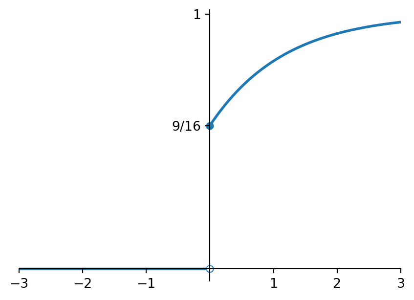
So, that was a bit of work, but our reward is that we have now found the following expression for the cdf of \(S\): \[F_S(x)=\begin{cases} 0 & \text{if } x<0 \\ 1-\frac{7}{16} e^{-\theta x} - \frac{\theta}{16} x e^{-\theta x} & \text{if } x \geq 0. \end{cases} \] You can maybe already see what is staring us in the face here, otherwise have a look at the plot in Figure 7.3: we have that \(F_S(0)=9/16\), while if we let \(x \uparrow 0\) then \(F_S(x) \uparrow 0\), i.e. \(F_S\) has a discontinuity in \(x=0\). So, \(F_S\) is not a piecewise constant function as the cdf of a discrete random variable would look like, and neither a continuous function (a property that the cdf of a continuous random variable has). So, \(S\) is neither a discrete nor a continuous random variable, it is an “other” one (cf. Section A.1.4)! This is not untypical for a compound distribution: if the \(X_i\)’s have a continuous distribution and \(\P(N=0)>0\), then \(S\) will always have this property!

Comp 2. How about an expectation, can we for instance compute the mean of \(S\) i.e. \(\E[S]\)? Yes we can! You may be tempted to think: “Oi, I have done all that work to find the cdf of \(S\), you know what, I’m just going to differentiate it so that I get the pdf and then it’s just a simple integral to get the mean!”. That’s very cute, but it’s WRONG! ;). This would be perfectly valid if \(S\) was a continuous random variable, but as we’ve just concluded in the final paragraph of Comp 1, \(S\) is not a continous random variable… Indeed, as we concluded, it is an “other” random variable, and we have from our earlier probability courses no tools at all to compute its mean! (cf. Section A.1.4).

So what do we do know? Panic? Grab the whiskey? No no, not to worry, after all we have the lovely Proposition 7.2 ii. :). If we want \(\E[S]\), then we should use the identity i.e. \(h(x)=x\) (so that \(h(S)=S\) eh). Using again that \(\text{Range}(N)=\{0,1,2\}\) and with probs given by Equation 7.23, we get from Proposition 7.2 ii that \[\begin{align*} \E[S] &= \sum_{n \in \text{Range}(N)} \E[S \, | \, N=n] \P(N=n) \\ &= \E[S \, | \, N=0] \cdot \frac{9}{16} + \E[S \, | \, N=1] \cdot \frac{6}{16} + \E[S \, | \, N=2] \cdot \frac{1}{16} \\ &= 0 \cdot \frac{9}{16} + \E[X_1] \cdot \frac{6}{16} + \E[X_1+X_2] \cdot \frac{1}{16}. \end{align*} \] And this is more straightforward to work out than the cdf above! All we need to do is observe that since the \(X_i\)’s have a common \(\text{Exp}(\theta)\) distribution, we have that (using Appendix B as needs be) \[\E[X_1]=\frac{1}{\theta} \quad \text{and} \quad \E[X_1+X_2]=\E[X_1]+\E[X_2]=\frac{2}{\theta}\] (for the second one, you could of course also use Equation 7.25 rather) so that we arrive at \[\E[S]=0 \cdot \frac{9}{16} + \frac{1}{\theta} \cdot \frac{6}{16} + \frac{2}{\theta} \cdot \frac{1}{16}=\frac{1}{2\theta}.\]

Figure 7.3: The cdf \(F_S\) of \(S\), with \(\theta=1\)

The strategy for analysing \(S\) that we have so far discussed in this section and captured in Proposition 7.2 can not only be used in specific cases such as in Example 7.5, it also allows us to derive some general expressions for the moment generating function (mgf) as well as the mean and variance of (essentially) any compound distribution!

Theorem 7.1 Let \(S\) be a random variable with a compound distribution as defined in Definition 7.1. Let \(M_N\) be the mgf of \(N\) and \(M_X\) the common mgf of the \(X_i\)’s. Then the mgf of \(S\), \(M_S\), is given by \[M_S(t) = M_N \Big( \log \big( M_X(t) \big) \Big) \tag{7.26}\] for any \(t \in \R\) for which \(M_X(t)<\infty\).

Further we have that \[\E[S]=\E[N] \E[X_1] \tag{7.27}\] (provided that the expectations in the right hand side are all well defined and finite) and \[\var(S)=\var(N) \big( \E[X_1] \big)^2 + \E[N] \var(X_1) \tag{7.28}\] (provided that the expectations and variances in the right hand side are all well defined and finite).

Some notes:

• If you’d like a reminder about mgf’s (=moment generating functions), see Section A.2.
• Recall (e.g. from Section A.2) that any mgf has co-domain \((0,\infty]:=(0,\infty) \cup \{\infty\}\). So if \(t \in \R\) is such that \(M_X(t)<\infty\) then \(M_X(t) \in (0,\infty)\), and then we can safely plug it into the logarithm, and the result of that operation into \(M_N\) i.e. the right hand side of Equation 7.26 is well defined. The end result could still be \(\infty\) though, depending on \(M_N\).
• In the proof below, we derive Equation 7.27 and Equation 7.28 via differentiation of Equation 7.26 (using the useful property Equation A.20 of mgf’s). In principle you could use the same route to derive higher moments of \(S\) as well if you need those (the algebra can get a bit annoying though…).

Proof. First for Equation 7.26. The idea is simple: we make both sides of the equation more explicit by plugging in the definitions of the mgf’s, and for the left hand side we also make use of Proposition 7.2 ii. Then we should hopefully have two expressions that look enough alike that we can see a clear path to proving that they’re indeed identical!

Fix some \(t \in \R\). For the left hand side of Equation 7.26 we can write \[\begin{align*} M_S(t) &= \E[e^{tS}] \\ &= \sum_{n \in \text{Range}(N)} \E[e^{tS} \, | \, N=n] \P(N=n), \end{align*} \tag{7.29}\] where the first equality is by def (cf. Section A.2) and the second uses Proposition 7.2 ii. For the right hand side of Equation 7.26, for any \(u \in \R\) fixed we have \[\begin{align*} M_N(u) &= \E[e^{uN}] \\ &= \sum_{n \in \text{Range}(N)} e^{un} \P(N=n), \end{align*} \] where the first eqaulity is again by def (cf. Section A.2) and the second uses the standard formula for the expectation of a function of a discrete random variable (cf. Equation A.9) with the choice \(h(x)=e^{ux}\). Plugging in the specific choice \[u=\log \big( M_X(t) \big)\] yields \[\begin{align*} M_N \Big( \log \big( M_X(t) \big) \Big) &= \sum_{n \in \text{Range}(N)} \exp \Big( n \log \big( M_X(t) \big) \Big) \P(N=n) \\ &= \sum_{n \in \text{Range}(N)} M_X(t)^n \P(N=n), \end{align*} \tag{7.30}\] where we used the little trick \[\exp(n \log(a))=\exp(\log(a^n))=a^n.\]

Now, if we compare Equation 7.30 with Equation 7.29, then we see that what remains to be done is showing that \[\E[e^{tS} \, | \, N=n]=M_X(t)^n \quad \text{for all } n \in \text{Range}(N).\] For the special case \(n=0\) (if indeed in this range) we get from Proposition 7.2 ii \[\E[e^{tS} \, | \, N=0]=e^{t \cdot 0}=1\] and of course also \(M_X(t)^0=1\). For any other \(n \in \text{Range}(N)\), again Proposition 7.2 ii yields \[\E[e^{tS} \, | \, N=n] = \E[e^{t (X_1+\ldots+X_n)}],\] but this right hand side is by def nothing but the mgf of \(X_1+\ldots+X_n\) in \(t\), and since the \(X_i\)’s are independent this boils down to the product of mgf’s (cf. Equation A.57) \[M_{X_1}(t) \cdot M_{X_2}(t) \cdot \ldots \cdot M_{X_n}(t).\] Further since the \(X_i\)’s are identically distributed they all have the same mgf, indeed the common mgf \(M_X\), so this product equals \(M_X(t)^n\). That’s it!

Now for Equation 7.27 and Equation 7.28. The key idea is again quite simple: now we have a relationship between the mgf’s of \(S\), \(N\) and the \(X_i\)’s, it is very tempting to use the fact that we can differentiate mgf’s to get our hands on moments, cf. Equation A.20 in Section A.2!

There is a bit of technical thinking needed as well though, because to Equation A.20 comes with a condition: a \(h>0\) exists so that for all \(t \in (-h,h)\) it holds that \(M_S(t)\) is well defined and finite. Let’s first assume this and later return to it.

Under this assumption, Equation A.20 yields for instance \[\E[S]=M_S'(0) \quad \text{and} \quad \E[S^2]=M_S''(0).\] Let’s work out what we get for these derivatives if we make use of Equation 7.26. Properly employing the chain rule gives \[M_S'(t)=M_N' \Big( \log \big( M_X(t) \big) \Big) \frac{M_X'(t)}{M_X(t)}.\] Plugging in \(t=0\), also using that any mgf evaluated in \(t=0\) yields \(1\) (immediate from its def, recall from Section A.2), gets us to \[M_S'(0)=M_N'(0) M_X'(0)\] which Equation A.20 readily translates to \[\E[S]=\E[N] \E[X_1].\] For the variance, use that \(\var(S)=\E[S^2]-(\E[S])^2\), and for the second moment we need here just turn to Equation A.20 to see that it equals \(M_S''(0)\). For this, differentiate Equation 7.26 a second time, and if you carefully work out the algebra you should arrive at Equation 7.28.

Finally, a quick word about how we can eliminate the need for the assumption we made for those of you interested (don’t worry about this for exam purposes). There’s a few ways here, including deriving it independently from the mgf result by using conditioning on \(N\) again, but we can also use a neat “truncation” argument which is commonly handy in Probablity Theory!

First consider any \(N\) and \(X_i\)’s that satisfy the weaker condition that the \(X_i\)’s are non-negative. Now define their “truncated” versions: set \(\widetilde{N}:=\min\{N,n\}\) for some \(n \geq 0\) and \(\widetilde{X}_i:=\min\{X_i,b\}\) for some \(b>0\), and \[\widetilde{S}:=\sum_{i=1}^\widetilde{N} \widetilde{X}_i.\] Then all these truncated random variables are bounded (\(0 \leq \widetilde{N} \leq n\) and \(0 \leq \widetilde{X}_i \leq b\)) and hence their mgf’s exist and are finite for all \(t \in \R\) (you can easily check this from the def of the mgf). Hence Equation 7.26 holds, all mgf’s in there are finite for all \(t \in \R\) and hence, by the work we did above, we get that Equation 7.27 and Equation 7.28 both hold for \(\widetilde{S}\). Further all expectations and variances appearing in Equation 7.27 and Equation 7.28 are finite.

The next step is to get rid of this truncation. Taking the limit for \(n \to \infty\) and \(b \to \infty\) and using the monotone convergence theorem, it follows that the first and second moments of the truncated random variables converge to the first and second moments of their original, “untruncated” versions. So the equalities Equation 7.27 and Equation 7.28 continue to hold for \(S\) as well. Be aware that we may now start to see infinities — it may well be true that Equation 7.27 and Equation 7.28 now yield \(\E[S]=\infty\) (which happens exactly if either \(\E[N]=\infty\) or \(\E[X_i]=\infty\)) and/or \(\var(S)=\infty\)!

Finally consider general \(N\) and \(X_i\)’s i.e. without any assumption at all. Defining \[X_i^{+}:=\max \{X_i,0\} \quad \text{and} \quad X_i^{-}:=\max \{-X_i,0\}\] we have that \(X_i=X_i^{+}-X_i^{-}\) and hence we can split up \[S=\sum_{i=1}^N X_i = \sum_{i=1}^N \left( X_i^{+}-X_i^{-} \right) = \sum_{i=1}^N X_i^{+} - \sum_{i=1}^N X_i^{-} =: S^{+}-S^{-}\] Now both \(S^{+}\) and \(S^{-}\) are of the type we discussed above and hence their expectations satisfy Equation 7.27. If these are both finite (which happens exactly if \(\E[N]<\infty\) and \(\E[X_i^{+}]<\infty\) and \(\E[X_i^{-}]<\infty\), or equivalently if \(\E[N]<\infty\) and \(\E[X_i]\) is well defined and finite) then by the triangle inequality \(\E[S]\) is also well defined and finite, and we can work out \[\begin{align*} \E[S] &= \E[S^{+}-S^{-}] \\ &= \E[S^{+}]-\E[S^{-}] \\ &= \E[N] \E[X_i^{+}] - \E[N] \E[X_i^{-}] \\ &= \E[N] \E[X_i^{+} - X_i^{-}] \\ &= \E[N] \E[X_i]. \end{align*} \] The second moment of \(S\) and hence variance is in the general case slightly more annoying but can be handled in a similar way.

Let’s conclude with a final quick example.

Example 7.6 Let’s revisit the compound distribution \(S\) from examples Example 7.3, Example 7.4 and Example 7.5 one last time.

Comp 1. In Example 7.5 we had already computed, taking the hard way via Proposition 7.2, that \[\E[S]=\frac{1}{2\theta}.\]

According to the above Theorem 7.1, in particular Equation 7.27, we should also be able to use that \[\E[S]=\E[N] \E[X_1].\] Indeed, using that the \(X_i\)’s have a common \(\text{Exp}(\theta)\) distribution, we have that \(\E[X_1]=1/\theta\) (using Appendix B if needs be). For the mean of \(N\), we could either work it out from the probabilities we saw in Example 7.3, namely \(\text{Range}(N)=\{0,1,2\}\) and \[\P(N=0)=\frac{9}{16}, \quad \P(N=1)=\frac{6}{16}, \quad \P(N=2)=\frac{1}{16}\] so that from Equation A.10 \[\E[N]=\sum_{n=0}^2 n \P(N=n)=\frac{1}{2},\] or alternatively we could use that \(N \sim \text{Binomial}(2,1/4)\) (from Example 7.4) to get \[\E[N]=2 \cdot \frac{1}{4}=\frac{1}{2}\] (recalling the mean of a Binomial distribution from Appendix B if needs be). So indeed \[\E[S]=\E[N] \E[X_1]=\frac{1}{2} \cdot \frac{1}{\theta}=\frac{1}{2\theta}.\]

Comp 2. Let’s also look at the mgf \(M_S\) of \(S\). Note that we could also have worked out this one using Proposition 7.2: by def (cf. Section A.2) \(M_S(t)=\E[e^{tS}]\), i.e. it is “just” an expectation of \(S\) and could attack it using Proposition 7.2 ii. However now we have Theorem 7.1 at our disposal, we may as well make optimal use of it! It tells us that \[M_S(t) = M_N \Big( \log \big( M_X(t) \big) \Big) \tag{7.31}\] for any \(t \in \R\) for which \(M_X(t)<\infty\), where \(M_N\) is the mgf of \(N\) and \(M_X\) the common mgf of the \(X_i\)’s. More good news: as discussed in Example 7.4, \(N \sim \text{Binomial}(2,1/4)\) and hence we can simply pick up its mgf from Definition 7.2: \[M_N(t) = \left( \frac{3}{4} + \frac{1}{4} e^t \right)^2 \quad \text{for all } t \in \R. \tag{7.32}\]

So the only hard work we really have to do is find \(M_X\). Fix some \(t \in \R\). Using that the \(X_i\)’s have a common \(\text{Exp}(\theta)\) distribution, we get from the def of mgf and Equation A.16 with the choice \(h(x)=e^{tx}\), where \(f_X\) is the common pdf of the \(X_i\)’s (recall from Appendix B if needs be) \[\begin{align*} M_X(t) &= \E[e^{tX_1}] \\ &= \int_{-\infty}^\infty e^{tx} f_X(x) \d x \\ &= \int_0^\infty e^{tx} \theta e^{-\theta x} \d x \\ &= \int_0^\infty \theta e^{-(\theta-t) x} \d x \\ &= \begin{cases} \frac{\theta}{\theta-t} & \text{if } t<\theta \\ \infty & \text{if } t \geq \theta \end{cases} \end{align*} \tag{7.33}\] (if the final step confuses you, have a look at Remark 7.2 below). Now, plugging Equation 7.33 and Equation 7.32 back into Equation 7.31, we find that \[M_S(t) = \left( \frac{3}{4} + \frac{\theta}{4(\theta-t)} \right)^2 \quad \text{for all } t \in (-\infty,\theta).\] See Figure 7.4 for a plot.

Finally, note that now we have the mgf available, we could obtain any moment of \(S\), i.e. \(\E[S^k]\) for any \(k=1,2,\ldots\), just by differentiating this mgf — recall from Equation A.20! Indeed this gives us also yet another way to compute \(\E[S]\): \[M_S'(t) = \frac{\theta}{2(\theta-t)^2} \left( \frac{3}{4} + \frac{\theta}{4(\theta-t)} \right)\] so \[\E[S]=M_S'(0)=\frac{1}{2\theta},\] reassuringly the same result as we found in Comp 1 above!

Figure 7.4: The mgf \(M_S\) of \(S\) for \(\theta=1\), with vertical asymptote at \(t=\theta=1\)

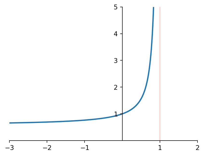
Remark 7.2. If you’re confused about the final step in the computation Equation 7.33, then recall that by construction, an integral with upperbound \(\infty\) is defined as a limit: \[\int_0^\infty g(x) \d x := \lim_{b \to \infty} \int_0^b g(x) \d x.\] Employing this, in Equation 7.33 we first do the integral for a finite \(b>0\), where we need to be aware that in the special case \(t=\theta\), \(e^{-(\theta-t) x}=1\): \[\int_0^b \theta e^{-(\theta-t) x} \d x = \begin{cases} \left. \frac{-\theta}{\theta-t} e^{-(\theta-t) x} \right|_{x=0}^{x=b}=\frac{-\theta}{\theta-t} \left( e^{-(\theta-t) b}-1 \right) & \text{if } t \not= \theta \\ \theta x \big|_{x=0}^{x=b} = \theta b & \text{if } t=\theta \end{cases} \] (if you didn’t realise that \(t=\theta\) is a special case, then alarm bells should go off when you write down the antiderivative: you’re dividing by \(0\) there if \(t=\theta\)!). Now we can take the limit for \(b\) to \(\infty\) to get the integral we need. Obviously \[\lim_{b \to \infty} \theta b=\infty\] and for \(t \not= \theta\) \[\lim_{b \to \infty} e^{-(\theta-t) b} =\begin{cases} 0 & \text{if } t<\theta \\ \infty & \text{if } t>\theta, \end{cases} \] yielding the expression given in the final step of Equation 7.33.

Remark 7.3. We have so far seen as many as three strategies to compute \(\E[S]\) for a compound distribution \(S\) (I know, desperately trying to give you some value for these tuition fees eh! ;)), namely:

• via Proposition 7.2 ii (cf. Example 7.5),
• via Equation 7.27 from Theorem 7.1 (cf. Comp 1 in Example 7.6),
• using Equation 7.26 from Theorem 7.1 to get to the mgf and then apply Equation A.20 (cf. Comp 2 in Example 7.6).

It’s maybe handy to agree on an overview of which one is best to use when:

• If you (only) need the mean and variance/second moment of \(S\), then just use Equation 7.27 and/or Equation 7.28 from Theorem 7.1.
• If you need the mgf specifically, or need higher order moments (third etc.) of \(S\), then use Equation 7.26 from Theorem 7.1 to get to the mgf and then apply Equation A.20 to get your hands on the higher order moments.
• If you need an expectation that is not a moment/the mgf, that is, \(\E[h(S)]\) for some function \(h\) that is not either \(h(x)=e^{tx}\) (because that would yield the mgf) or \(h(x)=x^k\) for some \(k=1,2,\ldots\) (because that would yield a moment), then use Proposition 7.2 ii.

7.4 Some exercises

NoteAbout the exercises

Each exercise has a (rough) indication of its difficulty, as follows:

*	easier: can be solved by (almost) only using relevant definitions/results,
**	medium: in addition to relevant definitions/results, needs a limited amount of work/creativity,
***	harder: in addition to relevant definitions/results, needs a larger amount of work/serious creativity,
💀	warning: might make your brain hurt! These are mainly intended to provide some extra challenge for those of you keen on that and are generally quite hard. You don't need to worry about these too much for exam purposes.

The exam consists of mostly ** and *** level questions, some *, and possibly at most a few marks worth of 💀.

A bit of preaching: it is an incredibly important part of the study process to try and work on the exercises as much as possible. To become a better mathematician/learn new maths (and also to get a good exam mark ;)), above all you need to do it. And yes, of course that includes falling over things, and making mistakes, and getting stuck, and getting frustrated — all part of the game and what you’re supposed to be doing! Your lecturers have done that as well and still do it. What matters is that you don’t let that discourage you and that you make good use of the help and resources available to help you develop your skills. As part of that, many exercises have a hint in a block like this:

NoteHint (click to view)

Hint!

These are trying to help you on your way if you don’t know where to start or to provide some ideas if you get stuck. In spirit of the above, always have a look at these first and try again before you look at the full solution. (These hints are an extra service that won’t be available in the exam I’m afraid ;).)

Of course, we have our classes and there’s office hours, email etc. as well — I’m at any time very happy to help you with any questions you may have, and you should please never feel that any question is “too dumb” to ask!

Full/detailed solutions for the exercises will become available, just immediately below the exercises, immediately after our tutorial hour (you may have to refresh the page).

Exercise 7.1 [**] Suppose that you are a risk manager facing a risk \(X \sim \text{Unif}(0,1)\).

1. You are considering entering a proportional sharing agreement, which leaves you with a fraction \(\alpha \in (0,1)\) of the risk. Determine the cdf and expectation of your part of the risk.
2. You are also considering to enter an excess of loss sharing agreement (so you are the cedant) with retention level \(K \in (0,1)\). Again determine the cdf and expectation of your part of the risk.
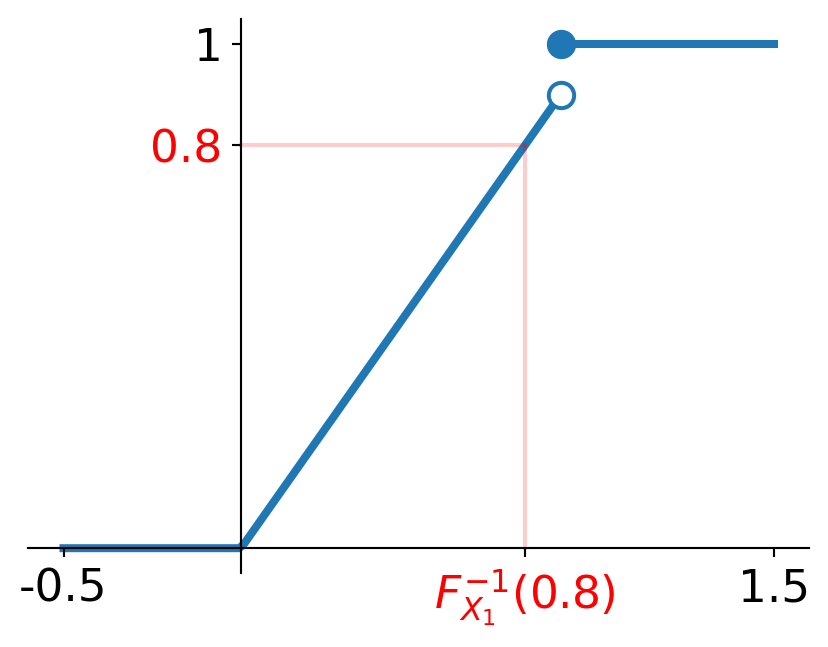
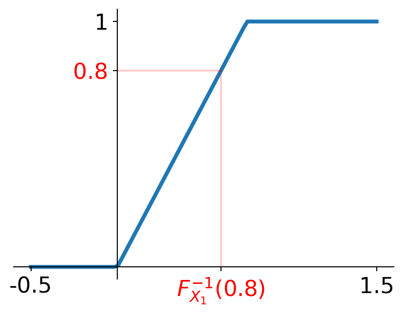
3. Suppose that in the excess of loss sharing agreement in part ii we set \(K=0.9\). You compare the benefit of both sharing agreements by comparing the Value-at-Risk at level \(0.8\) (cf. Definition 6.4) of the part of the risk you are responsible for. How do these VaR values for both agreements compare?

NoteHint (click to view)

For part i, recall the def of the agreement from Section 7.2.1: the part you’re left with is \(Y=\alpha X\). The expectation of \(Y\) is straightforward by using the standard linearity rule, and for its cdf just follow the same argument as in Equation 7.5.

For part ii, recall its construction from Section 7.2.2. You can follow exactly the same arguments as in Example 7.2!

For part iii, note that by def (cf. Definition 6.4), we need to evaluate the inverse of the cdf’s that we found in parts i and ii, each in the point \(y=0.8\). Recall that we discussed the concept of (generalised) inverse cdf’s in Section 2.2.1, and as we saw there: first sketch the graph of the cdf you want the inverse of and look at whether there is a unique \(x\)-value corresponding to \(y=0.8\). In both cases there is, so you can work out the inverse cdf’s in \(y=0.8\) just using the “classic” inverse technique!

TipFull solution (click to view)

In line with our notation in this chapter, in both parts i and ii we denote by \(Y\) the part of \(X\) that you are still responsible for with the relevant sharing agreement in place. Further recall (from Equation 2.2 e.g.) that the cdf of \(X\) is given by \[F_X(x)=\begin{cases} 0 & \text{if } x<0 \\ x & \text{if } x \in [0,1) \\ 1 & \text{if } x \geq 1. \end{cases} \tag{7.34}\]

For part i, as discussed in Section 7.2.1, under this agreement we have that \(Y= \alpha X\). So we immediately get that \[\E[Y]=\E[\alpha X]=\alpha \E[X]=\frac{\alpha}{2}\] (using that \(\E[X]=1/2\) as can be found in Appendix B e.g.). For the cdf \(F_{Y}\) of \(Y\) we can simply argue in the same way as in Equation 7.5: for any \(x \in \R\) \[\begin{align*} F_{Y}(x) &= \P(Y \leq x) \\ &= \P(\alpha X \leq x) \\ &= \P \left( X \leq \frac{x}{\alpha} \right) \\ &= F_X \left( \frac{x}{\alpha} \right) \\ &= \begin{cases} 0 & \text{if } x/\alpha<0 \\ x/\alpha & \text{if } x/\alpha \in [0,1) \\ 1 & \text{if } x/\alpha \geq 1 \end{cases} \\ &= \begin{cases} 0 & \text{if } x<0 \\ x/\alpha & \text{if } x \in [0,\alpha) \\ 1 & \text{if } x \geq \alpha, \end{cases} \end{align*} \tag{7.35}\] where in the fifth equality we plugged in Equation 7.34, and in the final step we write the case distinctions purely in \(x\) — not because that’s strictly necessary but it does look a bit neater!

As a little aside: can you recognise this cdf as a “well known” one?? Indeed, it shows that \(Y\) has a \(\text{Unif}(0,\alpha)\) distribution! And that’s intuitively appealing: if we think about \(X \sim \text{Unif}(0,1)\) as the result of the experiment in which we choose an element from the interval \((0,1)\) with all elements “equally likely”, then multiplying by \(\alpha\) naturally leads to that same experiment but only on the interval \((0,\alpha)\)!

For part ii, now for the excess of loss agreement. Recall that we discussed this one in Section 7.2.2. In particular, under this agreement we have that \(Y=\min\{X,K\}\), or equivalently \(Y=g(X)\) where the function \(g\) is given by \(g(x)=\min\{x,K\}\). For both the expectation and cdf we can follow the same ideas as in Example 7.2.

For the expectation, using the pdf \(f_X\) from Appendix B if needs be and the standard formula for the expectation of a function of a continuous rv (cf. Equation A.16) we can compute \[\begin{align*} \E[Y] &= \E[g(X)] \\ &= \int_{-\infty}^\infty g(x) f_X(x) \d x \\ &= \int_0^1 \min\{x,K\} \d x \\ &= \int_0^K x \d x + \int_K^1 K \d x \\ &= \frac{K^2}{2} + K(1-K) \\ &= K-\frac{K^2}{2}, \end{align*} \] where in the fourth equality we use that \(g(x)=x\) for \(x \in (0,K)\) and \(g(x)=K\) for all \(x \in [K,1)\) (it doesn’t matter which of the two cases you put \(x=K\) under!), exactly as we did in Example 7.2.

For the cdf, we can use not only exactly the same arguments as in Example 7.2, we can even use the same visuals (i.e. Figure 7.1) since we’re using exactly the same sharing agreement!

Indeed, for any \(x<K\) we get \[F_Y(x) = \P(Y \leq x) = \P(g(X) \leq x) = \P(X \leq x) = F_X(x),\] where the third equality uses Figure 7.1 (a). Note that since \(K \in (0,1)\), we see from Equation 7.34 that we get \(F_{Y}(x)=0\) for \(x<0\) while \(F_{Y}(x)=x\) for \(x \in [0,K)\).

For any \(x \geq K\) we get that \[F_{Y}(x) = \P(Y \leq x) = \P(g(X) \leq x) = 1,\] where the third equality now uses Figure 7.1 (b).

Hence altogether we arrive at \[F_{Y}(x)=\begin{cases} 0 & \text{if } x<0 \\ x & \text{if } x \in [0,K) \\ 1 & \text{if } x \geq K. \end{cases} \]

For part iii, recall that we defined the VaR in Definition 6.4 and that we did some comps with them in Exercise 6.4 e.g. From the def we have that \[\VaR_{0.8}(Y)=F_{Y}^{-1}(0.8).\] So, in particular we don’t need to specify \(F_{Y}^{-1}\) fully, all we need to know is what value it takes at \(0.8\)! As discussed in Section 2.2.1, you can always first sketch the graph of the cdf in question to visually inspect the situation.

• For the excess of loss agreement from part ii, with \(K=0.9\) the cdf of \(Y\) becomes \[F_{Y}(x)=\begin{cases} 0 & \text{if } x<0 \\ x & \text{if } x \in [0,0.9) \\ 1 & \text{if } x \geq 0.9. \end{cases} \] A sketch looks as in Figure 7.5 (a). Looking to find \(F_{Y}^{-1}(0.8)\), we look for corresponding \(x\)-values at the level \(y=0.8\). We see that there is a unique corresponding \(x\)-value, so we can just use the “classic” inverse and find the corresponsing \(x\)-value by solving \(0.8=F_{Y}(x)\): \[0.8=F_{Y}(x) \iff 0.8=x \iff x=0.8.\] So \[\VaR_{0.8}(Y)=F_{Y}^{-1}(0.8)=0.8.\]

• Next for the proprotional sharing agreement from part i, with the cdf of \(Y\) given by Equation 7.35, the sketch looks as in Figure 7.5 (b). Looking to find \(F_{Y}^{-1}(0.8)\), by the same arguments as just used we get that \[0.8=F_{Y}(x) \iff 0.8=\frac{x}{\alpha} \iff x=0.8 \alpha\] and hence \[\VaR_{0.8}(Y)=F_{Y}^{-1}(0.8)=0.8 \alpha.\]

So, recalling that \(\alpha \in (0,1)\), we see that the proprotional sharing agreement from part i yields a lower VaR value at level \(0.8\) than the excess of loss agreement from part ii does.

(a) \(F_Y\) for part i

(b) \(F_Y\) for part ii

Figure 7.5: Visually inspecting the cdf’s in this example

Exercise 7.2 [**/***] Recall the setting from Example 7.2: the risk is \(X \sim \text{Exp}(\theta)\) for some \(\theta>0\), and there is an excess of loss sharing agreement in place with retention level \(K>0\). Let \(Z\) be the part of the risk that the excess provider is responsible for.

1. Determine the cdf and expectation of \(Z\).
2. How could you actually have found that expectation in one short line??

NoteHint (click to view)

For part i, first recall from Equation 7.8 that we can write \(Z=g(X)\), where \(g(x) = \max\{x-K,0\}\). To compute the expectation and cdf of \(Z\), this is mathematically exactly the same problem as we discussed in Example 7.2 (and in Exercise 7.1). The only difference is that here we have a different function providing the connection between \(X\) and the random variable we are interested in. All the key ideas/strategy from Example 7.2 still apply though!

For part ii, the magic is to recall that in such a sharing agreement, a risk gets split into two parts and hence necessarily the sum of these two parts must be the original risk again — i.e. Equation 7.1!

TipFull solution (click to view)

For part i, recall from Equation 7.8 that we can write \(Z=g(X)\), where \[g(x) = \max\{x-K,0\}.\] We can (still) follow the same ideas as in Example 7.2, except that we now have a different function that connects \(Z\) to \(X\) than we had for connecting \(Y\) to \(X\).

For the expectation, using the standard formula for the expectation of a function of continuous rv’s (cf. Equation A.16) and the pdf \(f_X\) of \(X\) (use Appendix B if needs be): \[\begin{align*} \E[Z] &= \E[g(X)] \\ &= \int_{-\infty}^\infty g(x) f_X(x) \d x \\ &= \int_0^\infty \max\{x-K,0\} \theta e^{-\theta x} \d x \\ &= \int_K^{\infty} (x-K) \theta e^{-\theta x} \d x \\ &= \int_K^{\infty} x \theta e^{-\theta x} \d x - K \int_K^{\infty} \theta e^{-\theta x} \d x \\ &= Ke^{-\theta K} + \frac{1}{\theta} e^{-\theta K} - Ke^{-\theta K} \\ &= \frac{1}{\theta} e^{-\theta K}, \end{align*} \] where the fourth equality uses that \(\max\{x-K,0\}=0\) if \(x \leq K\) while \(\max\{x-K,0\}=x-K\) if \(x >K\), and the sixth uses integration by parts: \[\begin{align*} \int_K^{\infty} x \theta e^{-\theta x} \d x &= \left. -x e^{-\theta x} \right|_K^\infty + \int_K^{\infty} e^{-\theta x} \d x \\ &= K e^{-\theta K} + \left. \frac{-1}{\theta} e^{-\theta x} \right|_K^\infty \\ &= Ke^{-\theta K} + \frac{1}{\theta} e^{-\theta K}. \end{align*} \]

For the cdf, let’s use the same visual argument as in Example 7.2 to translate probs for \(Z\) into probs for \(X\): we sketch the graph of \(g\) and let \(x\) run along the vertical axis, from \(-\infty\) to \(\infty\) if you will. Cf. Figure 7.6. We see that we can distinguish two cases:

• If \(x<0\) (cf. Figure 7.6 (a)), then we see that the collection of \(w\)-values on the horizontal axis that satisfy \(g(w) \leq x\) is simply empty. I.e. it is not possible for \(g(X) \leq x\) to hold, and hence \[F_{Z}(x)=\P(Z \leq x)=\P(g(X) \leq x)=0.\]
• If \(x \geq 0\) (cf. Figure 7.6 (b)), then we see that \(w\) (on the horizontal axis) satisfies \(g(w) \leq x\) exactly if \(w \leq K+x\) i.e. \(g(X) \leq x\) holds if and only if \(X \leq K+x\). So \[F_{Z}(x)=\P(Z \leq x)=\P(g(X) \leq x)=\P(X \leq K+x)=F_X(K+x)=1-e^{-\theta (K+x)},\] where the final step uses the expression for the cdf \(F_X\) of \(X\) that we had already noted in Example 7.2, cf. Equation 7.9.

So in conclusion we arrive at the expression \[F_{Z}(x)=\begin{cases} 0 & \text{if } x<0 \\ 1-e^{-\theta (K+x)} & \text{if } x \geq 0. \end{cases} \] You may want to note that this cdf has a discontinuity at \(x=0\), so \(Z\) is not a continuous rv (nor is it discrete) — which we also already saw for \(Y\) in Example 7.2!

For part ii, the insight here is that if we denote by \(Y\) the part paid by the decant, then we have that \(X=Y+Z\) (cf. Equation 7.1). Now we have already worked out in Example 7.2 that \[\E[Y]=\frac{1}{\theta} \left( 1-e^{-\theta K} \right)\] and since \(X \sim \text{Exp}(\theta)\), \(\E[X]=1/\theta\) (use again Appendix B if needs be). So we immediately get that \[\E[Z]=\E[X-Y]=\E[X]-\E[Y]=\frac{1}{\theta}-\frac{1}{\theta} \left( 1-e^{-\theta K} \right)=\frac{1}{\theta} e^{-\theta K},\] indeed the same result as in part i! :).

Note: recall that the linearity rule \(\E[U+V]=\E[U]+\E[V]\) holds for any two rv’s \(U,V\), while e.g. the linearity rule \(\var(U+V)=\var(U)+\var(V)\) only holds if \(\cov(U,V)=0\) (which is e.g. the case if \(U\) and \(V\) are independent).

(a) Considering \(x<0\)

(b) Considering \(x \geq 0\)

Figure 7.6: A plot of \(g\)

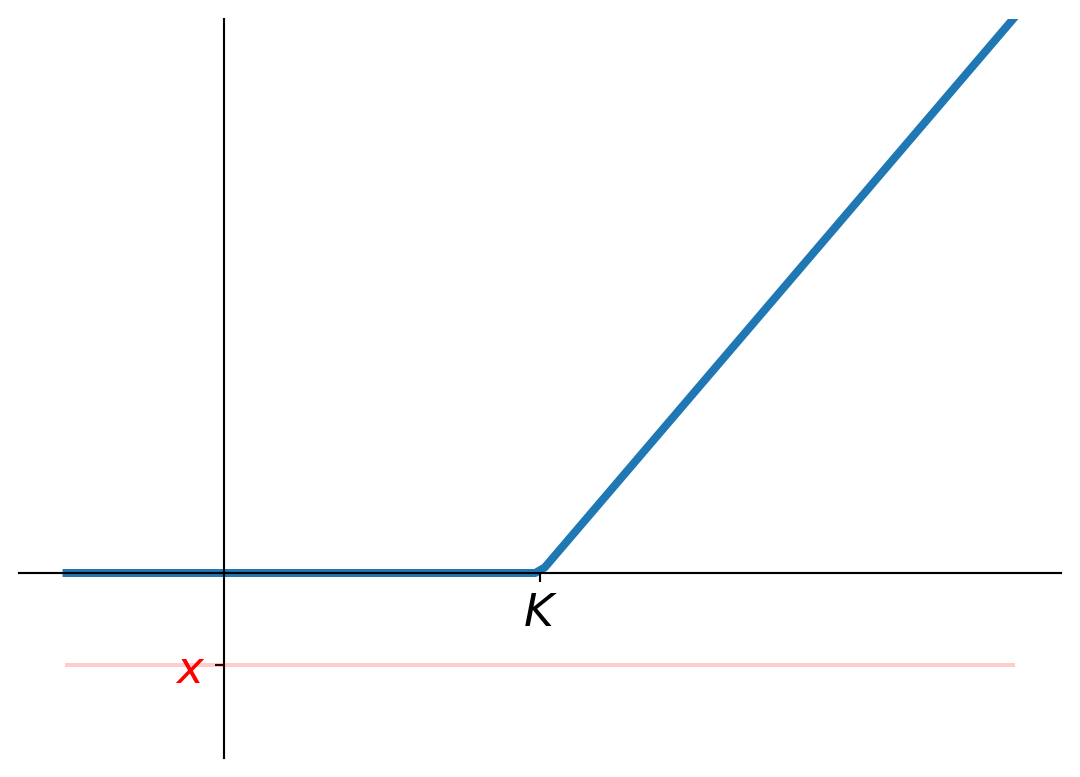
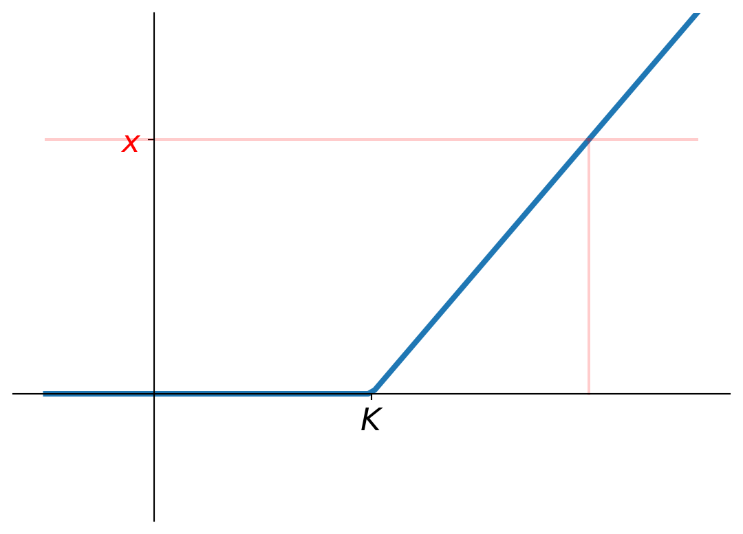
Exercise 7.3 [**/***] Note: this question explores a nice practical example in which techniques from this chapter and Chapter 6 naturally come together. It does make the whole working of this question quite long though! I really fully appreciate that the time you have to spend on this course is limited. On the other hand, I think (hope!) that it is nevertheless insightful and helpful to see this all at work. Of course, at the end of the day, working out all the comps/algebra/integrals etc. is not the important thing if you don’t have the time for that, the more important goal is that you understand how to solve the questions in principle!

Your phone is broken and you need to bring it in to a phone shop for repair. The cost of the repair is uncertain and is modelled, in hundreds of pounds, by a continuous random variable \(X\) with the pdf \(f_X\) given by \[f_X(x)=\begin{cases} (10-x)/50 & \text{if } x \in (0,10) \\ 0 & \text{otherwise.} \end{cases} \]

1. Explain why in this model, you won’t need to pay more than £1000.

2. The shop offers an arrangement in which they cover part of the cost, as follows:

   • if the cost turns out to be less than £500, then they cover 50% of the cost,
   • if the cost turns out to be more than £500, then they cover 50% of that £500 plus another 25% of the excess cost over £500.

   The shop does require a single premium payment from you in return. They compute this by means of the Variance premium principle with load factor \(\beta=0.1\) (applied to their risk). What is this premium?

3. So your options are to either accept the arrangement from part ii, or to be responsible for \(X\) by yourself. You decide to quantify your risk (in both cases) using the Conditional Tail Expectation with level \(0.9\) (recall from Definition 6.5). On that basis, which option is best? And does the result you find make sense to your mind?

   Hint: note that if you accept the agreement, then you need to pay the premium as well as the repair cost not covered by the shop! Express the sum of these as a single random variable.

NoteHint (click to view)

For part i, this is a one-liner — if you’re not sure, have a look at Equation A.18!

For part ii, recall from Section 6.2.1 that if we denote by \(Z\) the cost that the shop is responsible for, then the premium \(\pi(Z)\) is given by \[\pi(Z)=\E[Z]+0.1 \var(Z).\] So we need to find the expectation and variance of \(Z\). This is a novel form of risk sharing, i.e. not of the proportional or excess of loss form. So we’ll need to start from scratch. If you look at the discussion in Section 7.2, you see that the first step was always to find a function, say \(g\), expressing the relationship between this \(Z\) and the original \(X\) i.e. satisfying \(Z=g(X)\). If you think about it, then we should choose \[g(x)=\begin{cases} 0.5 x & \text{if } x \leq 5 \\ 1.25 + 0.25 x & \text{if } x>5. \end{cases} \] Now you can compute the expectation and variance of \(Z\) using that we’re given the pdf of \(X\) together with the standard formula for the expectation of a function of a continuous rv (cf. Equation A.16).

For part iii, lots of work to be done here! Observe that in order to compute the CTE, we need the pdf and VaR (cf. Definition 6.5), and in order to compute the VaR we need the (inverse) cdf (cf. Definition 6.4). If you have this strategy clear for yourself, then it is “just” a matter of diligently working through all the steps required.

First for the risk if you don’t take the arrangement i.e. simply \(X\). Its cdf can be found by integrating its pdf (recall from Equation A.12 e.g.) and yields \[F_X(x)=\begin{cases} 0 & \text{if } x \leq 0 \\ x/5-x^2/100 & \text{if } x \in (0,10] \\ 1 & \text{if } x>10. \end{cases} \] Using the visual route from Section 2.2.1 or otherwise, you can next derive that \[\VaR_{0.9}(X)=F_X^{-1}(0.9)=10-\sqrt{10}.\] Finally then it is matter of applying Definition 6.5 and work it out as in Example 6.4 e.g. to arrive at \[\cte_{0.9}(X) =10 - \frac{2}{3} \sqrt{10}.\]

Next for the risk, say \(R\), if you do take the arrangement. As in part ii, first connect \(R\) to \(X\). Now you should find (don’t forget about the premium payment!) that \(R=g(X)\) where the function \(g\) is given by \[g(x)=\begin{cases} \frac{1}{2} x+\frac{166}{100} & \text{if } x \leq 5 \\ \frac{3}{4}x+\frac{41}{100} & \text{if } x > 5. \end{cases} \] Next for the cdf of \(R\). Following our visual strategy as also used in Example 7.2 and Exercise 7.1 for instance, you should find that \[F_R(x)=\begin{cases} 0 & \text{if } x \leq \frac{83}{50} \\ -\frac{1}{25} x^2 + \frac{333}{625} x - \frac{48389}{62500} & \text{if } x \in \left(\frac{83}{50},\frac{104}{25} \right] \\ -\frac{4}{225} x^2 + \frac{1582}{5625} x - \frac{63181}{562500} & \text{if } x \in \left(\frac{104}{25},\frac{791}{100} \right] \\ 1 & \text{if } x > \frac{791}{100} \end{cases} \] (I know! Decimal numbers are also fine of course, just make sure to use enough of them to preserve enough accuracy throughout). You can then also easily compute the pdf of \(R\) by differentiating the cdf (recall from Section A.1.3 e.g.).

Now you have all the ingredients you need to follow the same steps as you followed above for \(X\) to work the CTE and ultimately arrive at \[\cte_{0.9}(R) \approx 6.33.\]

TipFull solution (click to view)

For part i, recall our standing convention that the range of a continous random variable is the set where its pdf is strictly positive (cf. Equation A.18). Hence in this case the range of \(X\) is the interval \((0,10)\), and since \(X\) gives the cost in hundreds of pounds, your repair cost can’t be more than \(10 \cdot £100=£1000\).

For part ii, let’s denote the part of \(X\) paid by the shop by \(Z\). This is a risk sharing arrangement as we’ve discussed in Section 7.2, but of a novel form (i.e. not propertional and neither excess of loss). Recall that in order to analyse the parts of such an arrangement, in this case \(Z\), the very first thing to do is to express the relationship between \(Z\) and \(X\) in the form \(Z=g(X)\) for the right function \(g\). If we have a go at this, then it tells us that if \(X \leq 5\), then \(Z=0.5 X\) while if \(X >5\), then \[Z=0.5 \cdot 5+0.25 (X-5)=1.25+0.25 X.\] That is, we have that \(Z=g(X)\) if we set \[g(x)=\begin{cases} 0.5 x & \text{if } x \leq 5 \\ 1.25 + 0.25 x & \text{if } x>5. \end{cases} \] Now on to seeing what we need from \(Z\) for the premium computation. Recall from Section 6.2.1 that it is given by \[\pi(Z)=\E[Z]+0.1 \var(Z) \tag{7.36}\] so we’ll need the expectation and variance of \(Z\). As \(X\) (and neither \(Z\)) does not have a “well known” distribution but we do have its pdf, we’ll just need to work these two out using the standard formulas for the expectation of a function of a continuous random variable (cf. Equation A.16): \[\begin{align*} \E[Z] &= \E[g(X)] \\ &= \int_{-\infty}^\infty g(x) f_X(x) \d x \\ &= \int_0^{10} g(x) \frac{10-x}{50} \d x \\ &= \int_0^5 0.5x \frac{10-x}{50} \d x + \int_5^{10} (1.25 + 0.25x) \frac{10-x}{50} \d x \\ &= \frac{1}{100} \left[ 5x^2-\frac{1}{3}x^3 \right]_0^5 + \frac{1}{50} \left[ 12.5x+0.625x^2-\frac{1}{12}x^3 \right]_5^{10} \\ &= \frac{5}{6} + \frac{35}{48} \\ &= \frac{25}{16} \end{align*} \] and similarly \[\begin{align*} \E[Z^2] &= \E[g(X)^2] \\ &= \int_{-\infty}^\infty g(x)^2 f_X(x) \d x \\ &= \int_0^{10} g(x)^2 \frac{10-x}{50} \d x \\ &= \int_0^5 0.25x^2 \frac{10-x}{50} \d x + \int_5^{10} (1.25 + 0.25x)^2 \frac{10-x}{50} \d x \\ &= \frac{125}{96}+\frac{275}{128} \\ &= \frac{1325}{384} \end{align*} \] (don’t get confused, we just used Equation A.16 with the choice \(h(x)=g(x)^2\)). So \[\var(Z)=\E[Z^2] - \big( \E[Z] \big)^2=\frac{1325}{384}- \left( \frac{25}{16} \right)^2=\frac{775}{768}\] and plugging this back into Equation 7.36 we ultimately find a premium of \[\pi(Z)=\frac{25}{16}+0.1 \frac{775}{768}=\frac{2555}{1536} \approx 1.66\] i.e. £166 (rounded to pounds). (Obviously, if you prefer to use decimal numbers in such working rather than fractions then that’s equally fine from an exam perspective, just make sure you use enough decimals to get an accurate enough end answer.)

For part iii, recall that we saw some examples of CTE computations in Example 6.4 and Exercise 6.4 for instance. We follow the same strategy as used there.

• First for the situation that you do not accept this agreement. Your risk is then just \(X\). To compute its CTE at level 0.9, we first need its VaR at level 0.9. And for the VaR we need the inverse cdf of \(X\). And for the inverse cdf, we first need the cdf itself of \(X\)! Ok. Ready??

  • The cdf. All we know about \(X\) is its pdf, so we’ll need to compute its cdf \(F_X\) from its fundamental relationship with the pdf, namely Equation A.12: \[F_X(x)=\int_{-\infty}^x f_X(y) \d y \quad \text{for all } x \in \R.\] For \(x \leq 0\) this gives \(\int_{-\infty}^x 0 \d y=0\), for \(x \in (0,10]\) we get \[\int_0^x \frac{10-y}{50} \d y = \frac{1}{5}x-\frac{1}{100}x^2\] and finally for \(x>10\) we find \(\int_0^{10} (10-y)/50 \d y=1\). So altogether: \[F_X(x)=\begin{cases} 0 & \text{if } x \leq 0 \\ x/5-x^2/100 & \text{if } x \in (0,10] \\ 1 & \text{if } x>10. \end{cases} \tag{7.37}\]
  • The VaR. We know from Definition 6.4 that \(\VaR_{0.9}(X)=F_X^{-1}(0.9)\). If you look at the expression for \(F_X\), then it is clear that it is a continuous function (as it should be, since \(X\) is a continuous rv, recall from Section A.1.3) and since it is strictly increasing for \(x \in (0,10)\), there is a unique \(x \in (0,10)\) corresponding to \(y=0.9\) which we can find using the “classic” inversion technique: \[0.9=F_X(x) \iff 0.9=\frac{x}{5}-\frac{x^2}{100} \iff -\frac{x^2}{100}+\frac{x}{5}-0.9=0.\] If you throw your standard formula for quadratic equations at this, you’ll find that the solutions are \(10 \pm \sqrt{10}\), and since we are looking for a solution \(x \in (0,10)\) it follows that we get \[\VaR_{0.9}(X)=F_X^{-1}(0.9)=10-\sqrt{10}.\] Note: in this argument we avoided the need for a graph of \(F_X\) by decuding its behaviour from its expression. However of course you can always go down the visual route Section 2.2.1 if you prefer and/or if you’re not certain!
  • The CTE. Finally then for the CTE! Recall its def from Definition 6.5 and for the working we can follow exactly the same strategy as in Example 6.4 for instance (the steps are also explained there): \[\begin{align*} \cte_{0.9}(X) &= \E[X \, | \, X>\VaR_{0.9}(X)] \\ &= \E[X \, | \, X>10-\sqrt{10}] \\ &= \frac{1}{\P(X>10-\sqrt{10})} \E \left[ \mathbf{1}_{\{ X>10-\sqrt{10} \}} X \right] \\ &= \frac{1}{0.1} \int_{10-\sqrt{10}}^{10} x \frac{10-x}{50} \d x \\ &= 10 \cdot \frac{1}{50} \cdot \int_{10-\sqrt{10}}^{10} 10 x -x^2 \d x \\ &= \frac{1}{5} \left[ 5x^2 - \frac{1}{3} x^3 \right]_{10-\sqrt{10}}^{10} \\ &= 10 - \frac{2}{3} \sqrt{10} \\ &\approx 7.89. \end{align*} \]

• Finally for the CTE in the case that you do accept this agreement. Your risk, let’s call it \(R\), can now be written as \(R=1.66+Y\), where \(1.66\) is the premium computed in part ii and \(Y\) denotes the amount you still have to pay with the arrangement from part ii in force. If we analyse \(Y\) in the same way as we did \(Z\) in part ii, then we see that if \(X \leq 5\) then we have that \(Y=0.5X\) while if \(X>5\) then \[Y=0.5 \cdot 5 + 0.75 (X-5)=0.75X-1.25.\] So (using fractions for optimal accuracy, you can of course also use decimal numbers rather — just keep in mind that because we need to go through quite a lot of calculations, you need to start with and maintain throughout enough decimals to get accurate enough end results): \[R=\frac{166}{100}+Y=\begin{cases} \frac{1}{2} X+\frac{166}{100} & \text{if } X \leq 5 \\ \frac{3}{4}X-\frac{5}{4}+\frac{166}{100}=\frac{3}{4}X+\frac{41}{100} & \text{if } X > 5 \end{cases} \] i.e. \(R=g(X)\) where the function \(g\) is given by \[g(x)=\begin{cases} \frac{1}{2} x+\frac{166}{100} & \text{if } x \leq 5 \\ \frac{3}{4}x+\frac{41}{100} & \text{if } x > 5. \end{cases} \] Let’s also already derive the cdf \(F_R\) and pdf \(f_R\) of R as we’ll need these later on. Following our visual strategy as also used in Example 7.2 and Exercise 7.1 for instance, sketching the graph of \(g\) we get that for any \(x \leq g(5)=104/25\) (cf. Figure 7.7 (a)) \[F_R(x)=\P(R \leq x)=\P(g(X) \leq x)=\P \left( X \leq 2x-\frac{83}{25} \right)=F_X \left( 2x-\frac{83}{25} \right)\] while for \(x>104/25\) (cf. Figure 7.7 (b)) \[F_R(x)=\P(R \leq x)=\P(g(X) \leq x)=\P \left( X \leq \frac{4}{3} x-\frac{41}{75} \right)=F_X \left( \frac{4}{3} x-\frac{41}{75} \right),\] and plugging this into Equation 7.37 we arrive at \[F_R(x)=\begin{cases} 0 & \text{if } x \leq \frac{83}{50} \\ \frac{1}{5} \left( 2x-\frac{83}{25} \right) - \frac{1}{100} \left( 2x-\frac{83}{25} \right)^2 = -\frac{1}{25} x^2 + \frac{333}{625} x - \frac{48389}{62500} & \text{if } x \in \left(\frac{83}{50},\frac{104}{25} \right] \\ \frac{1}{5} \left( \frac{4}{3} x-\frac{41}{75} \right) - \frac{1}{100} \left( \frac{4}{3} x-\frac{41}{75} \right)^2 = -\frac{4}{225} x^2 + \frac{1582}{5625} x - \frac{63181}{562500} & \text{if } x \in \left(\frac{104}{25},\frac{791}{100} \right] \\ 1 & \text{if } x > \frac{791}{100}. \end{cases} \] This also immediately gives us a formula for the pdf \(f_R\) of \(R\). Recall from Section A.1.3 e.g.: \(f_R\) is the derivative of \(F_R\) wherever that derivative exists, and any arbitrary value in points where \(F_R\) is not differentiable — the above expression (and/or the ‘kinks’ in the plot in Figure 7.8 (a)) shows that \(F_R\) is not differentiable in the points \(83/50\) and \(104/25\), we simply choose values there that give the most straightforward expression: \[f_R(x)=\begin{cases} 0 & \text{if } x \leq \frac{83}{50} \\ -\frac{2}{25} x + \frac{333}{625} & \text{if } x \in \left(\frac{83}{50},\frac{104}{25} \right] \\ -\frac{8}{225} x + \frac{1582}{5625} & \text{if } x \in \left(\frac{104}{25},\frac{791}{100} \right] \\ 0 & \text{if } x > \frac{791}{100} \end{cases} \] (see Figure 7.8 for a plot of these functions).

  Now let’s go and find that VaR and CTE!

  • The VaR. As above, from Definition 6.4 we have that \(\VaR_{0.9}(R)=F_R^{-1}(0.9)\), and following the usual visual route from Section 2.2.1 or otherwise we can see that \(F_R\) reaches the level \(0.9\) with a unique \(x\) from the interval \((104/25,791/100]\) i.e. that we can find by solving \[-\frac{4}{225} x^2 + \frac{1582}{5625} x - \frac{63181}{562500}=\frac{9}{10}.\] If you throw your quadratic equation solving skills at this guy, you’ll find the solutions \(791/100 \pm 75 \sqrt{10}/100\). Since we need a solution from the interval \((104/25,791/100]\), we can conclude that \[\VaR_{0.9}(R)=F_R^{-1}(0.9)=\frac{791}{100} - \frac{75 \sqrt{10}}{100} \approx 5.5383.\]
  • And now finally for the CTE! By the same arguments as above, we have that \[\begin{align*} \cte_{0.9}(R) &= \frac{1}{0.1} \int_{5.5383}^\infty x f_R(x) \d x \\ &= 10 \int_{5.5383}^\infty -\frac{8}{225} x^2 + \frac{1582}{5625} x \d x \\ &= 10 \cdot \left[ -\frac{8}{675} x^3 + \frac{1582}{11250} x^2 \right]_{5.5383}^{7.91} \\ &\approx 6.33. \end{align*} \]

• Conclusion: so, we have found that \(\cte_{0.9}(X) \approx 7.89\) while \(\cte_{0.9}(R) \approx 6.33\). Since the CTE is a measure of “riskyness” (recall from Section 6.3 e.g.), the lower it is, the better. Hence on this bases, it is better to choose \(R\) i.e. choose to accept the arrangement from part ii.

  Now, seeking a place in the sun to go sit down with a well deserved ice cream after all this work, sweat on our faces, can we understand/interpret why we got the result we did? Well, recall that the CTE is a risk measure i.e. it expresses how “risky” a risk is in terms of a real number, by focusing on the large values the risk can take. The arrangement in part ii has as benefit for us that it significantly reduces the (relatively) very large payment risk. One aspect to illustrate this: without arrangement the cost can be anything up to £1000, while with the arrangement in place it can cost at most £166 plus 50% of £500 plus 25% of another £500 i.e. £541. So indeed it makes sense that if we use the CTE as measure, that we prefer taking the arrangement.

  However, there are also good arguments against taking the arrangement. For instance, if you take it then no matter what happens, your cost will always be at least £166 because that’s the premium you’ll have to pay, even if the repair cost turns out to be only £10 or £20 or so… Another argument is that if you compare the expected costs then not taking the arrangement comes out better! After all \[\begin{align*} \E[R] &= \E[\pi(Z)+Y] \\ &= \pi(Z) + \E[Y] \\ &= \E[Z]+\E[Y]+ 0.1 \var(Z) \\ &= \E[Y+Z]+ 0.1 \var(Z) \\ &= \E[X]+ 0.1 \var(Z) \\ &> \E[X]. \end{align*} \]

  The reason for bringing this up here is just because this question is a nice practical application in which we can see in concrete action the point we made in general in Section 6.1 (and we encountered the same principle also in Section 5.1 e.g.): risks/random variables are complicated objects, and comparing them is not straightforward: often many criteria are possible that not all point to the same winner. The risk management way of thinking is to prioritise a particular criterion with a particular goal in mind. For instance, if your goal is to avoid large values, then the CTE is a good criterion to use, like we did in this question.

(a) Considering \(x \leq 104/25\)

(b) Considering \(x>104/25\)

Figure 7.7: A plot of \(g\)

(a) The cdf

(b) The pdf

Figure 7.8: The cdf and pdf of \(R\)

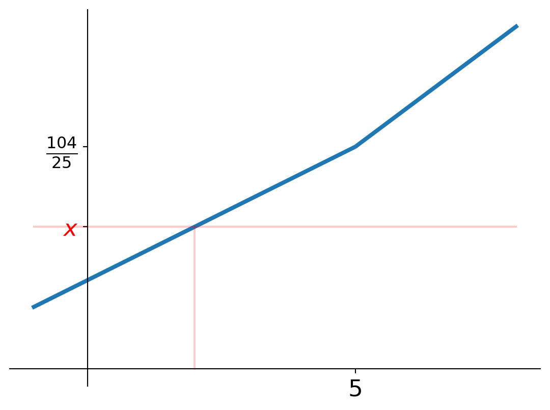
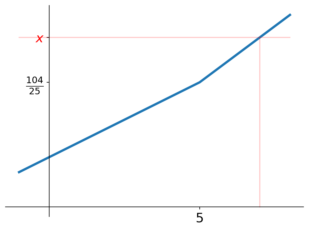
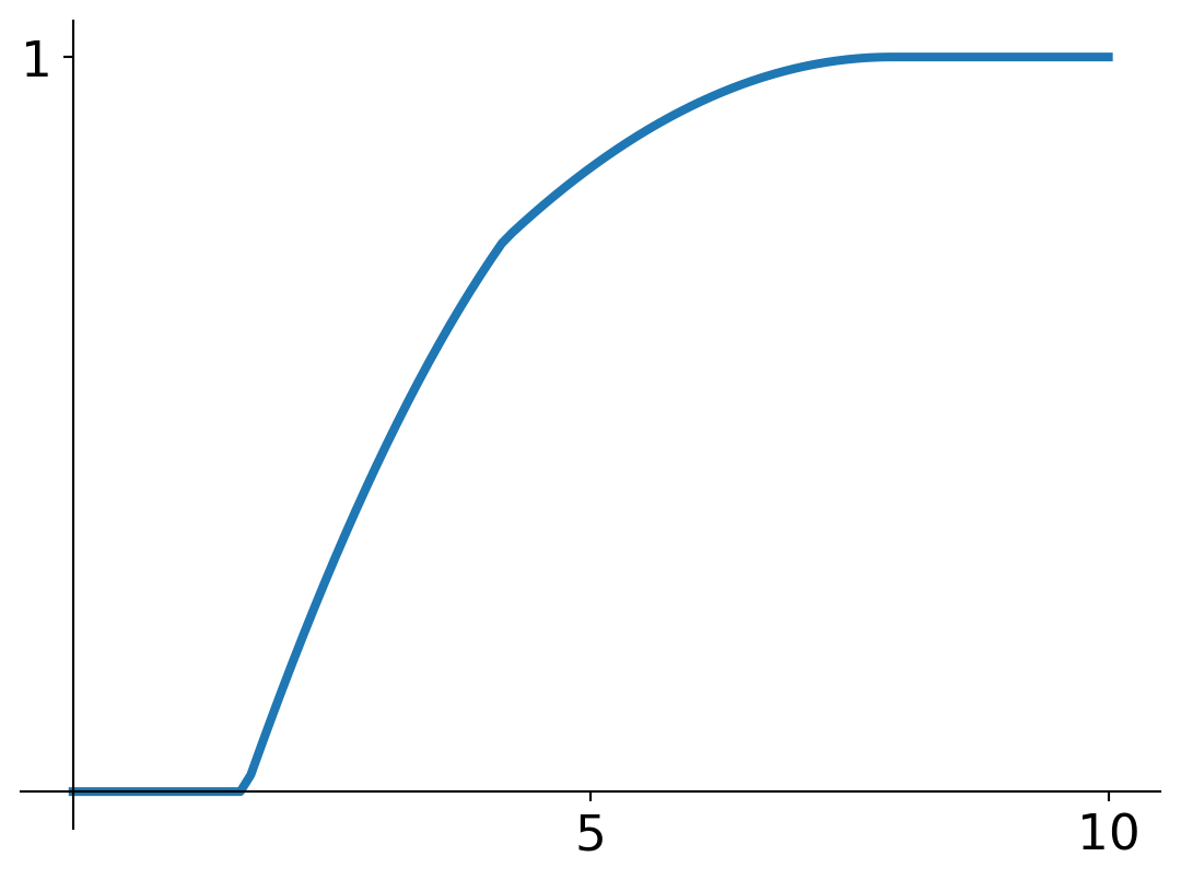
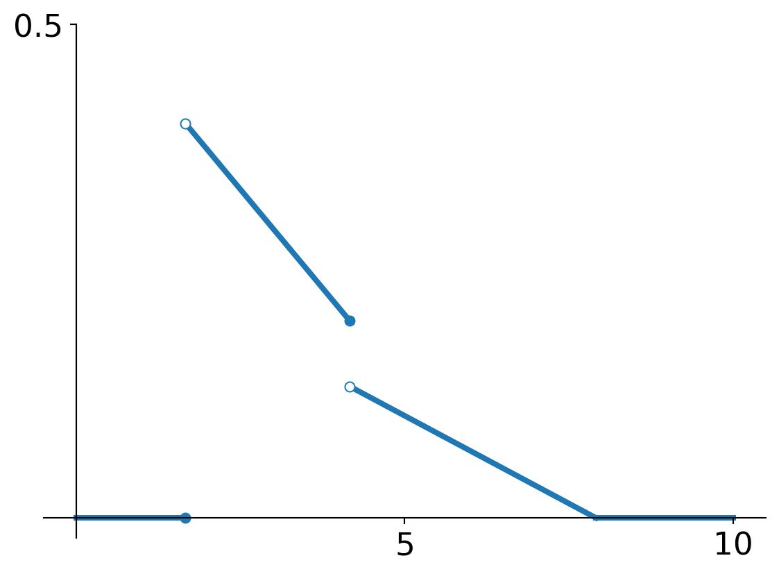
Exercise 7.4 [**] Of course, compound distributions as we introduced in Section 7.3 can be applied in many situations — here is a cute one involving our honourable course assistant Kevin the dog!

Kevin needs to be walked in principle every day, but if it rains the whole day both you and Kevin prefer to stay inside rather. From experience you know that it rains the whole day 20% of the time (which probably means that you live in Manchester). Further Kevin is quite fond of chasing squirrels and regularly catches one¹. You have kept count and found that during a walk, he catches none in 10% of the walks, one in 60% of the walks, and two in the remaining 30% of the walks.

¹ No panic, in real life the worst Kevin does to a squirrel he gets close to is bark very loudly — probably leaving it with a “peeeeep” in its ears for a while!

1. Compute the average number of squirrels Kevin catches during a week (=7 days).
2. Kevin’s all time weekly high currently stands at a very respectable 12 squirrels. What is the probability that Kevin will improve on his record next week?

Note: the goal of this exercise is to approach it via a compound distribution, although that’s not the only possible way (of course) — I hope it is nice/helpful to see them in action in a clear practical context. So even if you initially solved it otherwise, I’d really recommend to then still try and attack it using a compound distribution as well!

NoteHint (click to view)

First we’ll need to write down the compound distribution we want to be using. Recall from our discussions in Section 7.3 that it is a sum of i.i.d. random variables, and the number of terms that we sum up is (allowed to be) random as well. In this light it makes sense to see the number of squirrels caught in a week (say \(T\)) as a sum of i.i.d. random variables (say \(A_1, A_2, \ldots\)) each giving the number of squirrels caught during a walk, and with the number of terms being the number of days in a week Kevin actually gets to go for a walk (say \(D\)). This yields the expression \[T=\sum_{i=1}^D A_i,\] with the understanding that \(T=0\) if \(D=0\) (no walks, no squirrels!), and where in the right hand side we have the following distributions: \[A_i=\begin{cases} 0 & \text{with prob } 0.1 \\ 1 & \text{with prob } 0.6 \\ 2 & \text{with prob } 0.3 \end{cases} \] and \[D \sim \text{Binomial}(7,0.8).\]

For part i, recall the beautiful result that is Theorem 7.1!

For part ii, recall that for computing probs for a compound distribution we have established a “master” formula in Proposition 7.2 i. So pick that one up and use it to work out \(\P(T>12)\). It always looks like a daunting formula, but in this case all terms except for one of them equals \(0\) — and the one that isn’t \(0\) is not that hard to compute as well if you’re being a little bit smart about it! Crucial to keep in mind here: what is the largest value that each of the \(A_i\)’s can take??

TipFull solution (click to view)

There’s (of course) several ways to attack this question. It’s nice though to think about it from a compound distribution perspective. The idea is that the number of squirrels caught during each walk is a sequence of i.i.d. random variables, and then the number of these we need to add up to get to a weekly total is random as well as it depends on the how many not-rainy days we’re going to get.

That is to say, in line with Definition 7.1, if we denote by \(A_i\) the number of squirrels caught during the \(i\)-th walk of the week and by \(D\) the number of walks during the week, then we can express the total number of squirrels caught during a week, say \(T\), as \[T=\sum_{i=1}^D A_i,\] with the understanding that \(T=0\) if \(D=0\) (no walks, no squirrels!).

Further the \(A_i\)’s are i.i.d. with the following common distribution: \[A_i=\begin{cases} 0 & \text{with prob } 0.1 \\ 1 & \text{with prob } 0.6 \\ 2 & \text{with prob } 0.3, \end{cases} \tag{7.38}\] and by the logic also used in Section 7.3.1, \(D\) can be seen as the number of “successes” (=walks) from a sequence of seven (independent) repeats of the same experiment, each with “success” probability \(0.8\). So \[D \sim \text{Binomial}(7,0.8). \tag{7.39}\]

For part i, we’re asked to compute \(\E[T]\). From Theorem 7.1 we know that \[\E[T]=\E[D] \E[A_1].\] As we know well (or otherwise see Appendix B), \(\E[D]=7 \cdot 0.8=5.6\), Further we can compute (using the standard formula for the expectation of a discrete random variable, recall from Equation A.10 if needs be) \[\E[A_1]=0 \cdot 0.1 + 1 \cdot 0.6 + 2 \cdot 0.3=1.2.\] So plugging these in we find that \[\E[T]=5.6 \cdot 1.2 = 6.72.\]

For part ii, now we’re asked to compute \(\P(T>12)\). Computing probabilities for compound distributions is always a bit of an effort, but just carefully work out the “master” formula from Proposition 7.2 i as we also did in Example 7.5 e.g.! In this case, we clearly have that \(\text{Range}(D)=\{0,\ldots,7\}\), and hence Proposition 7.2 i yields \[\P(T>12)=\sum_{i=0}^7 \P(T>12 \, | \, D=i) \P(D=i). \tag{7.40}\] Now we need to work out all of the probabilities that appear in the right hand side. That could be nasty, but is luckily not too hard in this case!

Start by noting that it follows from Equation 7.39 that \[\P(D=i)=\binom{7}{i} \cdot 0.8^i \cdot 0.2^{7-i} \tag{7.41}\] (use Appendix B if you need a reminder). Further recall from Proposition 7.2 i that for the conditional probabilities appearing in Equation 7.40 we can argue as follows:

• For \(i=0\), \[\P(T>12 \, | \, D=0)=0,\] because conditional on \(D=0\) we have that \(T=0\) (no walks, no squirrels!) which is clearly not larger than 12.
• For \(i=1,\ldots,7\), \[\P(T>12 \, | \, D=i)=\P(A_1+A_2+\ldots+A_i>12).\] This is where the nasty part could be, but it’s actually not too bad if we stare at it for a bit. Note Equation 7.38 that each \(A_i\) has 2 as largest possible value, and so \(A_1+A_2+\ldots+A_i\) has \(2i\) as largest possible value. So in particular, for any \(i=1,\ldots,6\) it is impossible for \(A_1+A_2+\ldots+A_i\) to take a value larger than 12, which immediately gives us that \(\P(A_1+A_2+\ldots+A_i>12)=0\).

So, with the above considerations we see that Equation 7.40 simplifies to \[\begin{align*} \P(T>12) &= \sum_{i=0}^7 \P(T>12 \, | \, D=i) \P(D=i) \\ &= \P(T>12 \, | \, D=7) \P(D=7) \\ &= \P(A_1+A_2+\ldots+A_7>12) \cdot 0.8^7, \end{align*} \] where in the final step we also used Equation 7.41. So what is \(\P(A_1+A_2+\ldots+A_7>12)\)? Do we need to work out the distribution of \(A_1+A_2+\ldots+A_7\)?? :(. No we don’t need to if we’re just being a bit smart! Recalling the values that the \(A_i\)’s can take from Equation 7.38, we see that there are only two scenarios in which \(A_1+A_2+\ldots+A_7>12\) can happen:

• if \(A_1+A_2+\ldots+A_7=14\) i.e. \(A_1=A_2=\ldots=A_7=2\), which happens with probability \(0.3^7\).
• if \(A_1+A_2+\ldots+A_7=13\) i.e. six of the \(A_i\)’s take the value \(2\) and one of them takes the value \(1\). This happens with probability \[\binom{7}{1} \cdot 0.3^6 \cdot 0.6=7 \cdot 0.3^6 \cdot 0.6,\] where the factor \(\binom{7}{1}=7\) accounts for the fact that the one that takes the value \(1\) can be in seven different positions in the list \(A_1, A_2, \ldots, A_7\) (you’ll remember this from earlier Prob courses!).

So altogether we arrive at a prob only as small as \[\P(T>12)=\left( 0.3^7 + 7 \cdot 0.3^6 \cdot 0.6 \right) \cdot 0.8^7 \approx 0.0007,\] poor Kevin!

Not coming off my favourite blanket for that shit man.

Exercise 7.5 [💀] This is a cute and not very difficult question, but not crucial for exam prep etc. Recall that in Definition 7.2 we listed the moment generating function of a Binomial distribution and of a Poisson distribution. Derive from these expressions the well known formulas (e.g. as listed in Appendix B) for the mean and variance of a Binomial and a Poisson distribution.

NoteHint (click to view)

The key identity to use is Equation A.20 in Section A.2 (as also used in the proof of Theorem 7.1). Pick up the mgf’s in Definition 7.2, do your differentiation a bit carefully, and then you’ll indeed end up with these well known formulas!

TipFull solution (click to view)

It’s all about knowing the relationship to use and then it’s pretty straightforward. This relationship is the one we also used in the proof of Theorem 7.1, namely that by differentiating the mgf and plugging in \(t=0\) we can obtain moments of the distribution involved (cf. Equation A.20 in Section A.2).

First let \(N \sim \text{Binomial}(n,p)\) for some \(n \in \{1,2,\ldots\}\) and \(p \in (0,1)\). Then we know from Definition 7.2 that its mgf is given by \[M_N(t)= \left( 1-p+pe^t \right)^n \quad \text{for all } t \in \R.\] Hence (assuming \(n \geq 2\), you can do the case \(n=1\) separately) \[M_N'(t)=n \left( 1-p+pe^t \right)^{n-1} p e^t\] so that \(M_N'(0)=np\) and \[M_N''(t)=n (n-1) \left( 1-p+pe^t \right)^{n-2} p^2 e^{2t}+n \left( 1-p+pe^t \right)^{n-1} p e^t\] so that \(M_N''(0)=n(n-1)p^2+np\).

Hence from Equation A.20 we get that \[\E[N]=M_N'(0)=np\] and \[\begin{align*} \var(N) &= \E[N^2]-\big( \E[N] \big)^2 \\ &= M_N''(0)- \big( M_N'(0) \big)^2 \\ &= n(n-1)p^2+np - n^2 p^2 \\ &= np(1-p). \end{align*} \]

Next let \(N \sim \text{Poisson}(\lambda)\) for some \(\lambda>0\). Again appealing to Definition 7.2 we now get the mgf \[M_N(t)=\exp \left( \lambda (e^t-1) \right) \quad \text{for all } t \in \R\] with \[M_N'(t)=\lambda e^t \exp \left( \lambda (e^t-1) \right)=\lambda \exp \left( \lambda (e^t-1) +t\right)\] and \[M_N''(t)= \lambda \left( \lambda e^t+1 \right) \exp \left( \lambda (e^t-1) +t\right).\] So \(M_N'(0)=\lambda\) and \(M_N''(0)=\lambda (\lambda +1)\), so again from Equation A.20 \[\E[N]=M_N'(0)=\lambda\] and \[\begin{align*} \var(N) &= \E[N^2]-\big( \E[N] \big)^2 \\ &= M_N''(0)- \big( M_N'(0) \big)^2 \\ &= \lambda (\lambda +1) - \lambda^2 \\ &= \lambda. \end{align*} \]