3 Copulas 1: copulas & Sklar’s theorem

3.1 Why??

Ok then student risk manager, now we have Monte Carlo simulations under our belt as our first tool in our quest to understand and analyse future risks (recall: potential losses modelled by (non-negative) ranodm variables), in the next three chapters we will discuss copulas. Not the easiest topic I know from experience, but I hope you’ll nevertheless find them (somewhat) interesting and will see their value!

Quite commonly in our risk management adventures we need to assess a situation where the future uncertainty does not involve a single risk but several or even many rather. An investor typically invests in multiple types of assets/financial markets and is hence affected by the uncertainty in all of them. A construction manager is potentially affected by changes in material costs, by weather events, by personel changes etc. An insurance company’s bottom line depends on how many of its policyholder submit a claim, how large the claim sizes are, how many new policyholders it manages to recruit etc. Basically it’s everywhere!

As long as these risks can be reasonably assumed to be independent of each other then that’s generally not too much of a complication. But often enough that would a rather inappropriate, or even a misleading and dangerous assumption. Take for instance the investor. Different types of assets/financial markets tend to show clear dependencies: if we’re in an economic downturn then most assets tend to lose value at the same time. Or if OpenAI’s stock goes up because we’re all excited about chatting to a computer, then the stocks of key suppliers such as Nvidia (supplier of crucial hardware) tend to go up as well. Or take the insurance company. If an area suffers from a flooding damaging people’s houses, and you are the company who has sold many home insurances in the area, then you’ll have all these people knocking on your door/emailing you, many with a very substantial claim. That’s a bit of an oopsie if you didn’t properly account for such events in your modelling…

3.2 What is “dependence” again really actually hmm?

So we desperately need to talk about risks/“sources of uncertainty”/random variables that are not independent of each other. And, for clarity, note that this can come about in a more direct as well as more indirect way: the sources can influence each other directly (say, the number of blackjack games you win in the casino and the amount of money you go home with) or indirectly because they share some context that links them up say (for instance, the stock of a company in agriculture vs the stock of OpenAI — if the OpenAI stock was listed on the stock exchange of some civilisation of green men living on a far away planet then it would be sensible to assume independence, but as it is they are both subject to the same somewhat influential context namely the economical climate etc. on earth).

Not being independent hence means, a bit roughly speaking, that having some information about the outcome/result of one risk/random variable changes (your perception of) the characteristics/behaviour of the other risk/random variable. If you know that you’ll lose many blackjack games, then that knowledge significantly increases the likelihood you’ll return home from the casino with a pretty empty wallet (to a likely displeased partner!).

Mathematically, if we model our risks as random variables $X$ and $Y$, then as we know well (but cf. Section A.5 otherwise, in particular Equation A.53), they are independent if and only if for any $B_1, B_2 \subseteq \R$ with $\P(X \in B_1)>0$ and $\P(Y \in B_2)>0$ we have that \[\P(X \in B_1 \ \& \ Y \in B_2)=\P(X \in B_1) \P(Y \in B_2) \tag{3.1}\] or, equivalently, if (just by def of conditional probs, cf. Equation A.42) \[\P(Y \in B_2 \, | \, X \in B_1)=\P(Y \in B_2). \tag{3.2}\] In words: given any information about what happens to $X$ (because conditional on $X \in B_1$ for any $B_1$), all probabilities for $Y$ stay exactly the same i.e. the distribution of $Y$ does not change.

The logical opposite of this is then dependence i.e. there exist some sets $B_1, B_2 \subseteq \R$ with $\P(X \in B_1)>0$ and $\P(Y \in B_2)>0$ so that \[\P(Y \in B_2 \, | \, X \in B_1) \not= \P(Y \in B_2). \tag{3.3}\] That is: given the right piece of information about what happens to $X$ (namely that $X \in B_1$ happens), at least some probability for $Y$ changes i.e. the distribution of $Y$ changes at least somewhat.

Example 3.1 A very quick example to illustrate the subtlety above a little bit. Suppose that we roll two dice and denote the number of eyes on the first resp. second die by $X$ resp. $Y$. This is one of your stock examples of independent random variables of course, and you could easily check that Equation 3.1 and Equation 3.2 hold (for all sets $B_1, B_2 \subseteq \R$ with $\P(X \in B_1)>0$ and $\P(Y \in B_2)>0$ eh!).

Now let’s alter the experiment slightly: we add the rule that if the first die shows 6 eyes, then the second doesn’t have to be rolled and you get 6 eyes for free for the second as well. This creates some specific, rather minimal type of dependence:

if $X \not= 6$, then $Y$ (of course) still has nothing to do with $X$: equations Equation 3.1 and Equation 3.2 still hold (for any $B_2 \subseteq \R$) provided we plug in there any set $B_1 \subseteq \R$ that does not contain $6$.
but it breaks down for any set $B_1 \subseteq \R$ that does contain $6$, take for instance simply $B_1=\{6\}$ and (say) $B_2=\{3,4\}$. Then \[\P(Y \in B_2 \, | \, X \in B_1)=\P(Y \in \{3,4\} \, | \, X=6)=0\] while (using the Law of Total Probability, cf. Equation A.46) \[\begin{align*} \P(Y \in B_2) &= \P(Y \in \{3,4\}) \\ &= \P(Y \in \{3,4\} \, | \, X \not= 6) \P(X \not= 6) + \P(Y \in \{3,4\} \, | \, X = 6) \P(X = 6) \\ &= \frac{1}{3} \cdot \frac{5}{6} + 0 \cdot \frac{1}{6}=\frac{5}{18}, \end{align*} \] i.e. we’re now in the situation of Equation 3.3!

Note that in the above, it doesn’t matter which source we label $X$ and which $Y$ — indeed Equation 3.1 is perfectly symmetrical: $X$ and $Y$ are (in)dependent if and only if $Y$ and $X$ are (in)dependent.

Further keep in mind that in general, we are talking about probabilities for $X$ and $Y$ here. The above Example 3.1 is in a way extreme, in the sense that if $X=6$ then you know immediately for certain what value $Y$ will take. It could easily (and will typically) be more subtle, adjust the above example for instance as follows: if the first die shows 6 eyes then change the second die to a four-sided one. Then the certainty about what happens to $Y$ is gone, but there is still dependence.

3.3 Setting the scene for this chapter, and a motivational example

So, dependence is everywhere and is important for us. Let’s then open up and look in our mathematical toolbox: what we do have available in that section? Hmmm. A dry piece of gum, a dead mouse… Not much it seems? No hang on one of you will say, I found the correlation coefficient right in the corner there! Sure — but then that’s a pretty blunt tool: it measures something about dependence on a numerical scale but it can’t even tell the difference between independence (correlation coefficient $0$) and a number of forms of very strong dependence (plenty of such examples that also have correlation coefficient $0$)! We don’t actually even have a proper mathematical object to represent a particular dependency structure… But that’s where copulas come in! In the coming three chapters we’ll see what they are, how they can be used to represent dependency, and what insights they can give us about dependent random variables.

Throughout, we’ll limit ourselves to two random variables. Of course it’s also very interesting to look at dependency between more than two random variables. Most of the concepts and results we’ll discuss have a natural analogue for larger collections, but for the sake of simplicity of notation and easier visualisation etc. we’ll stick to two only.

Further, most of the time we’ll put the two random variables $X$ and $Y$ explicitly together in a pair $(X,Y)$. Recall the general model that we use for any probabilistic setting and that is always there even though we normally don’t (fully) specify it: some experiment with outcome space $\Omega$ is being done, an outcome $\omega \in \Omega$ is observed, and then $X$ takes the value $X(\omega) \in \R$ and $Y$ the value $Y(\omega) \in \R$, which are then samples/realisations/… of $X$ and $Y$. So both random variables, $X: \Omega \to \R$ and $Y: \Omega \to \R$, measure something of interest about the outcome of the experiment. For instance, we could randomly select a person in the Arndale Center (so $\Omega$ is the collection of all people present there) and measure both their height $X$ and weight $Y$ say (so $X: \Omega \to \R$ maps each person in the Arndale Center to their height, and $Y: \Omega \to \R$ to their weight)¹. By considering them as a pair $(X,Y)$, that model becomes: some experiment is done with outcome $\omega \in \Omega$, and then the pair $(X,Y)$ takes the value $(X(\omega),Y(\omega)) \in \R^2$, a point somewhere in the plane $\R^2$. This point is then a sample/realisation/… of the pair $(X,Y)$. See also Section A.3.

¹ Would you think that these two random variables are independent? Probably not right?

Of course it doesn’t make an actual difference whether we consider them as two separate random variables or as a pair, it’s just that the formulation as pair makes it more explicit that we consider them together and how they interact with each other. And it gives us more explicitly access to exisiting (and new) tools to study two random variables together, such as their joint cdf which unique characterises the distribution of the pair (which we intuitvely speaking understand as how the pair “behaves” in the plane i.e. which values it takes there with which probabilities).

Further, of course, also when we are working with a pair $(X,Y)$ nothing is stopping us from considering only $X$ on its own, or only $Y$ on its own, if we’d want to. Either of these are still random variables in their own right, with all the perks that come with that status, like that they each have a distribution, a cdf, etc. We just, in the context of a pair, normally add the word “marginal” to make explicit we are considering only one of the random variables from our pair: the marginal distribution or marginal cdf etc. of $X$ (or $Y$).

A quick overview of established facts and tools for dealing with pairs of random variables that we will use in this part of the course is provided in Section A.3. You have seen them all before in earlier Probability courses but nevertheless I’d strongly recommend to have a quick skim through so that you’re fully up to speed!

Example 3.2 Here is a quick example to further motivate just how influential dependency structures can be in how a pair of random variables behaves. Consider two pairs of random variables, as follows:

$(X_1,Y_1)$, where $X_1 \sim \text{Unif}(0,1)$, $Y_1 \sim \text{Unif}(0,1)$, and they are independent;
$(X_2,Y_2)$, where $X_2 \sim \text{Unif}(0,1)$ and $Y_2=1-X_2$. It’s not hard to see that $Y_2$ also has a $\text{Unif}(0,1)$ distribution. Indeed, since cdf’s uniquely determine distributions (recall from Section A.1.1) it is enough to show that the marginal cdf $F_{Y_2}(x)=\P(Y_2 \leq x)$ of $Y_2$ has the required form (cf. Equation 2.2). To see this, take any $x \in [0,1]$ and work out the marginal cdf of $Y_2$ by using that $Y_2=1-X_2$: \[\begin{align*} \P(Y_2 \leq x) &= \P(1-X_2 \leq x) \\ &= \P(X_2 \geq 1-x) \\ &= 1-\P(X_2 \leq 1-x) \\ &= 1-(1-x) \\ &= x, \end{align*} \] where we used Equation 2.2 for the fourth equality as well.

If you would naively compare these two pairs, then you might say “well $X_1$ has the same marginal distribution as $X_2$, and $Y_1$ has the same marginal distribution as $Y_2$. So surely the pair $(X_1,Y_1)$ has the same distribution as the pair $(X_2,Y_2)$ i.e. they behave in the same way?” The answer is that they don’t! In fact they very much don’t! Below we will show this, twice even. Note that you were right about the fact that the marginal distributions are the same between the two pairs, however that’s not the whole story. What makes the difference between the pairs is how completely different the dependency structures are: independence in the case of $(X_1,Y_1)$ vs a form of “full” dependence in the case of $(X_2,Y_2)$!

Approach 1. First for a quick and (somewhat) dirty approach. Intuitively, if we want to compare the distributions of two pairs, i.e. how they “behave” in terms of the values that they tend to take in $\R^2$, then why not just generate/simulate a lot of such values i.e. samples for each pair, plot these, and compare these two plots? That works!

We can underpin this intuition as follows. Recall from our Monte Carlo simulation adventure, in particular Equation 1.7, the following. For any $B \subseteq \R^2$, if we produce $n$ (‘large’) samples from a pair $(X,Y)$ then the (exact) probability that $(X,Y)$ ends up in $B$ can be approximated by the ratio of samples that end up in $B$: \[\P((X,Y) \in B) \approx \frac{\text{Nr samples in } B}{n}. \tag{3.4}\] So if $(X_1,Y_1)$ and $(X_2,Y_2)$ would have the same distribution, i.e. (by def, cf. Equation A.21) $\P((X_1,Y_1) \in B)=\P((X_2,Y_2) \in B)$ for any $B \subseteq \R^2$, then Equation 3.4 implies that no matter which region in these plots we focus on (“for any $B \subseteq \R^2$”), we should count approximately the same number of samples in that region in either plot.

Now, Listing 3.1 shows a bit of R code to produce such plots. Note that these plots show the unit square, where both pairs take their values, as part of the larger plane $\R^2$. Note how very different they look! More precisely in line with the argument from the previous paragraph: you can easily find plenty of regions where the sample count between both plots is very different. Take the square with vertices $(0,0)$ and $(1/4,1/4)$ for instance. No samples at all in there in the plot of $(X_2,Y_2)$, but quite a few in the plot of $(X_1,Y_1)$.

As a little extra/aside: in the plot of $(X_2,Y_2)$, all the samples seem to be concentrated on the line $y=1-x$. Makes sense? Well yes, very much so, just look back at how we have defined the pair $(X_2,Y_2)$! That definition also makes clear that it is impossible for a sample of $(X_2,Y_2)$ to end up in the square with vertices $(0,0)$ and $(1/4,1/4)$. After all, any point $(x,y)$ in there satisfies $x \leq 1/4$ and $y \leq 1/4$. But if a sample $(x,y)$ from $(X_2,Y_2)$ satisfies $x \leq 1/4$, then $y=1-x \geq 3/4>1/4$!

Approach 2. Now for a more theoretical (and exact) approach. Recall (cf. Section A.3.1) that the distribution of a pair is fully characterised by its joint cdf. So let’s work out the joint cdf’s of our pairs so that we can compare them. Note that in both cases, it is enough to consider the joint cdf on the unit square $(0,1)^2$ in $\R^2$ since that’s where both pairs take their values (as discussed in Lemma A.2 iii). Further recall that the cdf $F$ of a $\text{Unif}(0,1)$ distributed random variable satisfies (cf. Equation 2.2) \[F(x)=x \quad \text{for all } x \in (0,1) \tag{3.5}\] (that’s the only bit of that cdf that we need here).

Now, for the joint cdf $F_{X_1,Y_1}$ of $(X_1,Y_1)$ we get for any $x,y \in (0,1)$ \[F_{X_1,Y_1}(x,y)=F_{X_1}(x) F_{Y_1}(y)=xy, \tag{3.6}\] where we first use that $X_1$ and $Y_1$ are independent (cf. Section A.5) and then Equation 3.5.

For the joint cdf $F_{X_2,Y_2}$ of $(X_2,Y_2)$ we have to work a little bit harder. There are no obvious shortcuts here, and so the best can do is to simply start from the very def of the joint cdf (cf. Section A.3.1), plug in what we know about $(X_2,Y_2)$, and hope that we end up somewhere nice! This gives for any $x,y \in (0,1)$ \[\begin{align*} F_{X_2,Y_2}(x,y) &= \P(X_2 \leq x \ \& \ Y_2 \leq y) \\ &= \P(X_2 \leq x \ \& \ 1-X_2 \leq y) \\ &= \P(X_2 \leq x \ \& \ X_2 \geq 1-y) \\ &= \begin{cases} 0 & \text{if } x \leq 1-y \\ \P(X_2 \in [1-y,x]) & \text{if } x > 1-y \end{cases} \\ &= \begin{cases} 0 & \text{if } x \leq 1-y \\ x+y-1 & \text{if } x > 1-y, \end{cases} \end{align*} \tag{3.7}\] where in the second equality we plugged in the def of $Y_2$, in the fourth we use that if $x \leq 1-y$ then it is impossible for $X_2$ to satisfy both $X_2 \leq x$ and $X_2 \geq 1-y$, and in the final one that $X_2 \sim \text{Unif}(0,1)$ so \[\P(X_2 \in [1-y,x])=\P(X_2 \leq x)-\P(X_2 \leq 1-y)=x-(1-y)\] (by Equation 3.5). If you’re confused that we wrote “$\P(X_2 \leq 1-y)$” rather than “$\P(X_2 < 1-y)$”, then recall that they are identical, cf. Equation A.14.

So, as conclusion of approach 2: comparing Equation 3.6 with Equation 3.7 they are indeed wildly different functions, confirming that $(X_1,Y_1)$ and $(X_2,Y_2)$ have different distributions!

Listing 3.1: R code for producing some scatter plots — you’ll remember the R commands from Chapter 2

3.4 Copulas & Sklar’s theorem

The key take away from Section 3.3, and in particular Example 3.2, was: if we want to understand the distribution of a pair $(X,Y)$, then it’s not enough to look at the marginal distributions of $X$ and $Y$ only, the dependency structure is also crucially important. Putting what we know so far together in a handy visual, like an amateur detective frantically drawing lines between pictures of the potential suspects on a board²: we know that the joint cdf of $(X,Y)$ uniquely characterises its distribution and vice versa (cf. Section A.3.1), and the marginal distributions of $X$ and $Y$ (uniquely characterised by the marginal cdf’s) plus the dependency structure are the three ingredients that are in some way (at this point unknown how exactly!) mixed together to make up the distribution/joint cdf. So: \[\begin{align*} \text{Distribution}&& && \text{Joint} && && \text{Marginal cdf } F_X, \text{ plus} \\ \text{of the pair} && \longleftrightarrow && \text{cdf} && \longleftrightarrow && \text{marginal cdf } F_Y, \text{ plus}\\ (X,Y) && && F_{X,Y} && && \text{dependence between $X$ and $Y$} \end{align*} \tag{3.8}\] This visual is the big picture we constantly keep in mind in this part of course! Note that the second “$\leftrightarrow$” works in the same way as when you mix amounts of red, green and blue together to create any other colour³: on the one hand, any colour can be (uniquely) decomposed into a certain amount of red, of blue, and of green (“$\rightarrow$”). On the other hand, pick a certain amount of red, of blue, and of green and mix them together to produce a colour (“$\leftarrow$”). If you change the amount of any of the red, blue or green then you will change the colour that you get, and similarly if you make any change to one or more of the marginal cdf of $X$, marginal cdf of $Y$ and the dependency structure then you change the joint cdf⁴.

² Too much Diet Coke, sorry

³ Only works with light, don’t try this with paint unless you’re a big fan of mud!

⁴ Well this is the exact truth as long as we’re working with continuous marginal cdf’s at least, as we’ll see in Theorem 3.1

Our goal in this section is essentially to fully understand this picture. For this we have two things to do: firstly to put some kind of mathematical object in place that represents the still somewhat opaque “dependence between $X$ and $Y$”, and secondly to figure out how the second “$\leftrightarrow$” in Equation 3.8 exactly works: how exactly do we go from joint cdf to marginal cdf $F_X$ & marginal cdf $F_Y$ & dependence between $X$ and $Y$, and the other way around?

Starting with the former: it turns out that the right mathematical object to use for representing dependency structures is a copula. It is nothing but a function of two variables, with as domain the unit square and with certain properties.

Definition 3.1 A copula is a function $C: [0,1]^2 \to [0,1]$ satisfying the following conditions:

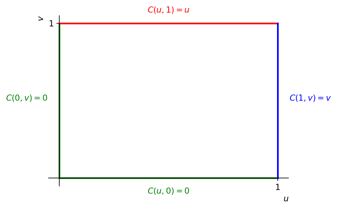
$C(u,0)=0$ and $C(0,v)=0$ for all $u,v \in [0,1]$,
$C(u,1)=u$ and $C(1,v)=v$ for all $u,v \in [0,1]$,
For all $0 \leq u_1 \leq u_2 \leq 1$ and $0 \leq v_1 \leq v_2 \leq 1$ it holds that \[C(u_2,v_2)-C(u_1,v_2)-C(u_2,v_1)+C(u_1,v_1) \geq 0.\]

Here’s an important observation about that definition.

Remark 3.1. Note that Definition 3.1 i & ii fully specify the values of a copula $C$ on the boundary of its domain $[0,1]^2$ i.e. for any point $(u,v)$ where $u$ is either $0$ or $1$, or $v$ is either $0$ or $1$. Cf. Figure 3.1.

So any two copulas can only differ on the open unit square $(0,1)^2$ i.e. for points $(u,v)$ with $u \in (0,1)$ and $v \in (0,1)$. On this open unit square a copula can do anything, as long as it respects Definition 3.1 iii. That one looks like a quite unpleasant one to have to check, but luckily we won’t have to do that very often!

Figure 3.1: Visualising the domain of a copula $C$, and how it is defined on the boundary of its domain

Obviously at this point we have absolutely no feel whatsoever for how these guys could possibly represent dependency structures between random variables, but we’ll get there! For now, let’s go with the flow and think: any copula i.e. function $C$ as defined in Definition 3.1 represents a possible dependency structure of a pair $(X,Y)$, and vice versa any possible dependency structure that a pair $(X,Y)$ can have is represented by a copula $C$. So, a one-to-one correspondence between the collection of all copulas on the one hand and the collection of all possible dependency structures. This means that we can update our big picture from Equation 3.8 to \[\begin{align*} \text{Distribution}&& && \text{Joint} && && \text{Marginal cdf } F_X, \text{ plus} \\ \text{of the pair} && \longleftrightarrow && \text{cdf} && \longleftrightarrow && \text{marginal cdf } F_Y, \text{ plus}\\ (X,Y) && && F_{X,Y} && && \text{a copula $C$ describing the dependency} \end{align*} \tag{3.9}\]

On to the second main question: how does the second “$\leftrightarrow$” in Equation 3.9 exactly work, i.e. given some joint cdf $F_{X,Y}$, how do we “decompose” it into the three components marginal cdf $F_X$, marginal cdf $F_Y$ and copula $C$ exactly? And vice versa, given some choices for a marginal cdf $F_X$, a marginal cdf $F_Y$ and a copula $C$, how exactly do we bolt these together to produce the resulting joint cdf $F_{X,Y}$? The answers here are (largely) provided by the seminal Sklar’s theorem (if you’re interested in a proof, see e.g. McNeil, Frey, and Embrechts (2015)):

Theorem 3.1 (Sklar’s theorem) Recall that copulas were defined in Definition 3.1. We have the following.

For any pair $(X,Y)$ with joint cdf $F_{X,Y}$ and marginal cdf’s $F_X$ and $F_Y$, there exists a copula $C$ so that \[F_{X,Y}(x,y)=C(F_X(x),F_Y(y)) \quad \text{for all } x,y \in \R. \tag{3.10}\] Further, if $F_X$ and $F_Y$ are continous functions, then $C$ is unique.
Given a copula $C$ and two cdf’s $F_1, F_2$, the function $F: \R^2 \to [0,1]$ defined as \[F(x,y)=C(F_1(x),F_2(y)) \quad \text{for all } x,y \in \R \tag{3.11}\] is the joint cdf of some pair $(X,Y)$ with marginal cdf’s $F_1$ and $F_2$.

Some notes:

Recall that a continuous random variable is guaranteed to have a continuous cdf, while for a discrete random variable it is guaranteed to be discontinous rather. For “other” random variables the cdf may or may not be continuous. Cf. Section A.1.
Here’s how Sklar’s theorem underpins the second “$\leftrightarrow$” in Equation 3.9, at least for continuous marginal cdf’s:
- “$\rightarrow$”: given some pair $(X,Y)$ with joint cdf $F_{X,Y}$, first extract the marginal cdf’s $F_X$ and $F_Y$ (cf. Lemma A.2 ii). If these are continuous, then statement i guarantees that there is a unique copula $C$ so that Equation 3.10 holds. This is then the copula of $(X,Y)$ describing its dependency structure.
- “$\leftarrow$”: take any continuous cdf’s $F_1, F_2$ and a copula $C$. Using statement ii above, we can construct the joint cdf of some pair $(X,Y)$, of the form Equation 3.11. Then applying statement i above to that joint cdf shows that this construction is unique in the sense that only this particular copula could have resulted in this particular joint cdf.
If we’re dealing with a situation in which the marginal cdf’s are not both continuous then it’s all a bit less nice: there is not necessarily a unique copula anymore for a given pair/joint cdf. The main use case of copulas is for continuous marginals, so we don’t need to worry about this too much. Vague bottom line: in this situation, a pair does not have a uniquely defined dependency structure, at least not when we associate dependency with copulas (or, if you consider a dependency structure intrinsic to a pair, then in this situation the association between copulas and dependency structures is not one-to-one).

Note that despite all the glory of Sklar’s theorem, it doesn’t actually provide us with an explicit procedure for extracting the copula from a pair $(X,Y)$ with continuous marginals: statement i says that it uniquely exists and gives the relationship Equation 3.10 but it’s not very obvious how to actually extract $C$ from that. We’ll resolve this in a moment, but first a simple enough example where Sklar’s theorem is all we need:

Example 3.3 Take a pair $(X,Y)$ where $X$ and $Y$ have continuous marginal cdf’s $F_X$ and $F_Y$, and are independent of each other (one of the pairs in Example 3.2 was of this type). In this case, as we know well (cf. Section A.5), the joint cdf $F_{X,Y}$ satisfies \[F_{X,Y}(x,y)=F_{X}(x) F_{Y}(y) \quad \text{for all } x,y \in \R. \tag{3.12}\] Now, according to Theorem 3.1 i, there exists a unique copula $C$ describing this dependency structure (i.e. independence!) and it is characterised by \[F_{X,Y}(x,y)=C(F_X(x),F_Y(y)) \quad \text{for all } x,y \in \R. \tag{3.13}\] Hmmm. Which copula i.e. function $C: [0,1]^2 \to [0,1]$ could possible work here?? ;). Well indeed, plugging Equation 3.12 into Equation 3.13 it must hold that \[C(F_X(x),F_Y(y))=F_{X}(x) F_{Y}(y) \quad \text{for all } x,y \in \R. \tag{3.14}\] i.e. $C$ must simply return the product of both its arguments. That is, the function $C: [0,1]^2 \to [0,1]$ given by \[C(u,v)=uv.\] Here it is, look at it sitting there like the good boy that it is — your first actual real life explicit example of a copula! It describes the (somewhat trivial) dependency structure that is independence and is therefore fittingly called the independence copula.

Note that we didn’t explicitly check that this function $C$ is actually a copula i.e. satisfies conditions of Definition 3.1. We don’t actually need to, for two reasons: first, we have here enough info to deduce this indirectly (though it needs a somewhat subtle ;) argument, see Remark 3.2 below), and secondly, the next result we’ll discuss allows us to draw this conclusion without further ado.

Remark 3.2. Following up on the final paragraph in Example 3.3, here is the argument. Key is the continuity of $F_X$ and $F_Y$. Due to this continuity and the well known limiting behaviour of cdf’s (cf. Equation A.5), as we let $x$ and $y$ run through the whole of $\R$, $F_X(x)$ and $F_Y(y)$ will each hit every possible value in $(0,1)$. This allows for the following argument. Fix any $u,v \in (0,1)$. Then there exist some $x \in \R$ and $y \in \R$ so that $F_X(x)=u$ and $F_Y(y)=v$. Fix these as well. Recalling that we need Equation 3.14 to hold and plugging in there the specific $x$ and $y$ we had fixed we get that \[C(F_X(x),F_Y(y))=F_{X}(x) F_{Y}(y) \implies C(u,v)=uv.\]

Since this argument works for any $u,v \in (0,1)$, it follows that the only function $C: (0,1)^2 \to [0,1]$ for which Equation 3.13 holds is $C(u,v)=uv$. Now, according to Theorem 3.1 i, there exists a copula that satisfies Equation 3.13. This copula is in particular also a function from $(0,1)^2$ to $[0,1]$ (ignoring the boundary of $[0,1]^2$). So it must be the case that $C(u,v)=uv$ is identical to the copula that Theorem 3.1 i tells us about, at least on the domain $(0,1)^2$. You can readily check that $C(u,v)=uv$ satisfies the boundary behaviour prescribed in Definition 3.1 i and ii, so in fact $C(u,v)=uv$ is identical to the copula that Theorem 3.1 i tells us about on the whole of $[0,1]^2$. Hence in particular $C(u,v)=uv$ is a copula.

This argument also highlights the underlying reason for the difficulties with non-uniqueness of copulas in the case of non-continuous marginals as highlighted in Sklar’s theorem. Indeed say for simplicity that $X$ and $Y$ are both discrete random variables taking possible values/with range $\{a_1,\ldots,a_n\}$. Then $F_X$ and $F_Y$ are piecewise constant functions, only hitting the following values in $(0,1)$: $F_X(a_1), F_X(a_2), \ldots, F_X(a_n)$ resp. $F_Y(a_1), F_Y(a_2), \ldots, F_Y(a_n)$. So looking for a copula $C$ characterised by Theorem 3.1 i i.e. \[F_{X,Y}(x,y)=C(F_X(x),F_Y(y)) \quad \text{for all } x,y \in \R, \tag{3.15}\] we see that now this equation only specifies what values $C(u,v)$ should have for \[\begin{align*} u &\in \{ F_X(a_1), F_X(a_2), \ldots, F_X(a_n) \} \\ & \text{ and } v \in \{ F_Y(a_1), F_Y(a_2), \ldots, F_Y(a_n) \}, \end{align*} \tag{3.16}\] not for any other $u,v \in (0,1)$! Hence, Equation 3.15 is in this situation not demanding enough to uniquely specify a copula: any two that have the correct values in the specific points $(u,v) \in (0,1)^2$ given by Equation 3.16 but with different values elsewhere in $(0,1)^2$ would equally well satisfy Equation 3.15!

So, Sklar’s theorem Theorem 3.1 tells us that for a pair $(X,Y)$ with continuous marginal cdf’s $F_X$ and $F_Y$ a unique copula $C$ describing the dependency structure exists, and that it satisfies the relationship Equation 3.10, but otherwise doesn’t give us anything in the way of an explicit expression for what $C$ would look like. For this purpose we have the following lovely

Proposition 3.1 Let $(X,Y)$ be a pair of random variables with joint cdf $F_{X,Y}$ and continuous marginal cdf’s $F_X$ and $F_Y$, so that it has a unique copula $C: [0,1]^2 \to [0,1]$ describing its dependency structure (cf. Theorem 3.1). Then \[C(u,v)=F_{X,Y} \left( F_X^{-1}(u),F_Y^{-1}(v) \right) \quad \text{for all } u,v \in (0,1). \tag{3.17}\]

Some notes:

Note that in Equation 3.17 we only consider $u,v \in (0,1)$, so we don’t include the boundary of the domain of $C$ i.e. points $(u,v)$ with $(u,v)$ with $u \in \{0,1\}$ and/or $v \in \{0,1\}$. This no problem, because the fact that $C$ is a copula fully specifies its values there, cf. Remark 3.1. And the advantage of this formulation is that we need to know the inverse marginal cdf’s $F_X^{-1}$ and $F_Y^{-1}$ only on $(0,1)$.
The inverse marginal cdf’s used in Equation 3.17 may have to be generalised inverses as we already introduced in Chapter 2, cf. Definition 2.1. Even though $F_X$ and $F_Y$ are continuous, they may still have constant/flat bits.

Proof. Define $C: [0,1]^2 \to [0,1]$ by Equation 3.17 and by the usual values a copula has on the boundary of $[0,1]^2$ (cf. Remark 3.1). It is sufficient to show that Equation 3.10 holds, because then we can use the same argument as in Remark 3.2 to conclude that this $C$ must be the copula Theorem 3.1 i is alluding to. To show that Equation 3.10 holds we consider two cases.

Case 1. First consider some $x,y \in \R$ for which $F_X(x) \in \{0,1\}$ or $F_Y(y) \in \{0,1\}$ (or both) holds. Then Equation 3.10 holds essentially trivially. For instance, if $F_X(x)=0$ then \[C \left( F_X(x),F_Y(y) \right)=C \left( 0,F_Y(y) \right)=0\] (the final equality by Definition 3.1 i). And also \[\begin{align*} 0 &\leq F_{X,Y}(x,y) \\ &= \P(X \leq x \ \& \ Y \leq y) \\ &\leq \P(X \leq x) \\ &= F_X(x)=0, \end{align*} \] where we only use the definitions of (joint) cdf’s and that the event $\{X \leq x \ \& \ Y \leq y\}$ is a subset of the event $\{X \leq x\}$. So both sides of Equation 3.10 equal $0$. The other possibilities follow similarly.

Case 2. Now take some $x,y \in \R$ that we haven’t covered yet, i.e. with $F_X(x) \in (0,1)$ and $F_Y(y) \in (0,1)$. Using the expression Equation 3.17 for our $C$, we get that \[C \left( F_X(x),F_Y(y) \right)=F_{X,Y} \left( F_X^{-1}(F_X(x)),F_Y^{-1}(F_Y(y)) \right)\] and hence to arrive at Equation 3.10 it remains to show that \[F_{X,Y} \left( F_X^{-1}(F_X(x)),F_Y^{-1}(F_Y(y)) \right)=F_{X,Y}(x,y). \tag{3.18}\] Obviously it is very tempting here to think that we can just use the general principle that $f^{-1}(f(x))=x$ and be done with it — however don’t forget, as mentioned in Proposition 3.1, that we may be working with the generalised inverse here and then things are not so simple, recall from Lemma 2.1!

That makes things a bit fiddly I’m afraid, sorry. :(. We claim that, no matter what, we can legally replace $F_X^{-1}(F_X(x))$ by $x$ and $F_Y^{-1}(F_Y(y))$ by $y$ in Equation 3.18. To see this, we can do them both separately. If $F_X$ is not flat/constant in $x$, then $F_X^{-1}(F_X(x))=x$ by Lemma 2.1 i. If $F_X$ is flat/constant around $x$ then there exist $a \leq x \leq b$ so that $F_X(z)=F_X(x)$ for all $z \in [a,b]$ while $F_X(z)<F_X(x)$ for $z<x$ and $F_X(z)>F_X(x)$ for $z>b$. And then $F_X^{-1}(F_X(x))=a$ (cf. Definition 2.1). But this doesn’t actually matter in Equation 3.18, exactly because $F_X$ being flat on $[a,b]$ means that $X$ has zero probability of taking a value in $[a,b]$. In algebra: \[\begin{align*} F_{X,Y} \left( F_X^{-1}(F_X(x)),F_Y^{-1}(F_Y(y)) \right) &= \P \left( X \leq F_X^{-1}(F_X(x)) \ \& \ Y \leq F_Y^{-1}(F_Y(y)) \right) \\ &= \P \left( X \leq a \ \& \ Y \leq F_Y^{-1}(F_Y(y)) \right) \\ &= \P \left( X \leq x \ \& \ Y \leq F_Y^{-1}(F_Y(y)) \right) \\ & \qquad - \P \left( X \in (a,x] \ \& \ Y \leq F_Y^{-1}(F_Y(y)) \right) \\ &= \P \left( X \leq x \ \& \ Y \leq F_Y^{-1}(F_Y(y)) \right) \\ &= F_{X,Y} \left( x,F_Y^{-1}(F_Y(y)) \right), \end{align*} \] where the fourth equality follows from the flatness of $F_X$ on $[a,b]$: \[\begin{align*} 0 &\leq \P \left( X \in (a,x] \ \& \ Y \leq F_Y^{-1}(F_Y(y)) \right) \\ &\leq \P(X \in (a,x]) \\ &= \P(X \leq x)-\P(X \leq a) \\ &= F_X(x)-F_X(a)=0. \end{align*} \] The replacement of $F_Y^{-1}(F_Y(y))$ by $y$ in Equation 3.18 is justified in the same way.

With Proposition 3.1 we now have a very useful tool to go find some more examples of copulas! We conclude this chapter with seeing it in action, and a remark about the nature of copulas.

Example 3.4 First let’s pick up the situation from Example 3.3 one more time: $(X,Y)$ with continuous marginal cdf’s $F_X$ and $F_Y$, and $X$ and $Y$ independent of each other. We had in that example already found an expression for the corresponding copula by making an educated guess. Let’s confirm that we could also have dealt with this one by making use of Proposition 3.1: for any $u,v \in (0,1)$ \[\begin{align*} C(u,v) &= F_{X,Y} \left( F_X^{-1}(u),F_Y^{-1}(v) \right) \\ &= F_X \left( F_X^{-1}(u) \right) F_Y \left( F_Y^{-1}(v) \right) \\ &= uv, \end{align*} \] where we used that due to independence, we have that $F_{X,Y}(x,y)=F_X(x) F_Y(y)$ for all $x,y \in \R$ (for clarity: we used that here with $x=F_X^{-1}(u)$ and $y=F_Y^{-1}(v)$) and we also used Lemma 2.1 ii (very convenient that $F_X$ and $F_Y$ are continuous no!). Here is indeed our independence copula again!

Let’s do one more. Recall the following pair we encountered in Example 3.2: $(X,Y)$ where $X \sim \text{Unif}(0,1)$ and $Y=1-X$, which yields $Y \sim \text{Unif}(0,1)$ as well. We had also already derived an expression for the joint cdf $F_{X,Y}$ (cf. Equation 3.7): for any $x,y \in (0,1)$ \[F_{X,Y}(x,y) = \begin{cases} 0 & \text{if } x \leq 1-y \\ x+y-1 & \text{if } x > 1-y. \end{cases} \tag{3.19}\]

For working out the copula of this pair using Proposition 3.1, first note that since $X$ and $Y$ each have a (marginal) $\text{Unif}(0,1)$ distribution, their marginal cdf’s satisfy (cf. e.g. Equation 2.2) \[F_X(x)=F_Y(x)=x \quad \text{for all } x \in (0,1) \tag{3.20}\] and hence their inverses are simply $F_X^{-1}: (0,1) \to \R$ and $F_Y^{-1}: (0,1) \to \R$ given by \[F_X^{-1}(y)=F_Y^{-1}(y)=y \quad \text{for all } y \in (0,1). \tag{3.21}\] (Aside: don’t get confused here. The starting point is: in order to work out Equation 3.17, we need to know what $F_X^{-1}$ and $F_Y^{-1}$ are. For the purposes of Equation 3.17 we need to be able to plug any $u \in (0,1)$ into $F_X^{-1}$ and any $v \in (0,1)$ into $F_Y^{-1}$, so we need to find these two inverses with domain $(0,1)$. Conveniently, for our purposes $(0,1)$ is always the domain of an inverse cdf, recall the discussion in Section 2.2.1. And though Equation 3.22 is only part of the expression for $F_X=F_Y$, it is the only part that we need: it shows that for any $y \in (0,1)$, there is a unique solution $x$ to the equation $F_X(x)=F_Y(x)=y$ and so we can just use the classic inverse here, yielding Equation 3.29.)

So Equation 3.17 now gives that the copula $C$ of this pair is given by, for all $u,v \in (0,1)$: \[\begin{align*} C(u,v) &= F_{X,Y} \left( F_X^{-1}(u),F_Y^{-1}(v) \right) \\ &= F_{X,Y} \left( u,v \right) \\ &= \begin{cases} 0 & \text{if } u \leq 1-v \\ u+v-1 & \text{if } u > 1-v. \end{cases} \end{align*} \tag{3.22}\] Note that we may also write this as the convenient one liner: \[C(u,v)=\max\{u+v-1,0\} \quad \text{for all } u,v \in (0,1). \tag{3.23}\]

So, after the independence copula, here is our second explicit example of a copula! :). This is also a rather special one. After all $(X,Y)$ has a rather extreme dependency structure: there is “full negative dependence” in the sense that $X$ fully determines $Y$ and/or $Y$ fully determines $X$ (“full”) and a (relatively) large value of $X$ comes with a (relatively) small value of $Y$ (“negative”). Apparently that type of dependency is characterised by the copula Equation 3.22, which is called the countermonotonicity copula. Indeed this observation can be formulated in more general terms, cf. Exercise 3.4.

Remark 3.3. This remark gives some more context about the fundamental how & why of copulas — don’t worry about the second part (the “why copulas” bit) for exam purposes though!

So, in what way exactly do copulas represent dependency structures? I mean, at the end of the day a copula is just a function (cf. Definition 3.1). And if somebody writes down such a function i.e. \[C(u,v)=\text{[some expression in $u$ and $v$]},\] how do you know what dependency structure it actually represents? If somebody would give you Equation 3.23, would you be able to tell immediately that that expression represents “full negative dependence”? No, right?

The truth is that the link between a copula and the dependency structure it represents is rather opaque. Copulas act as unique identifiers of dependency structures in a similar way as that in a supermarket, every product has a unique barcode on it (the bit on the packaging that you scan in the self checkout): such a barcode uniquely identifies a product in the supermarket i.e. every product has its own barcode, but if somebody would show you a barcode only, you wouldn’t (without further investigations) know what product belongs to it in the same way as that when somebody shows you a copula you wouldn’t (without further investigations) know what dependency structure it represents.

So in order to get more feel for what dependency structure a certain copula represents we need to do these “further investigations”, and we’ll embark on that adventure in the coming two chapters.

Ok, but then why copulas as unique identifiers of dependency structures, why not something else? Well just because you actually very naturally end up with copulas! The thinking that leads to copulas happens in two steps.

Step 1. For the moment, only consider the collection $\mathcal{A}$ of all pairs of random variables $(X,Y)$ in which both $X$ and $Y$ have a (marginal) $\text{Unif}(0,1)$ distribution. Since within this class the marginals are always the same, the only way any two pairs can have different distributions and hence different joint cdf’s is by having different dependency structures (cf. Equation 3.9). That is, for any two pairs $(X_1,Y_1)$ and $(X_2,Y_2)$ within this class, $(X_1,Y_1)$ and $(X_2,Y_2)$ have the same dependency structure if and only if they have the same joint cdf.

So, we decide to simply use the joint cdf itself as unique identifier: every possible joint cdf within this class corresponds to exactly one possible dependency structure and vice versa. Indeed, if you look again closely, you’ll notice that the collection of all copulas i.e. of functions as defined in Definition 3.1 is nothing but the collection of all possible joint cdf’s of pairs in $\mathcal{A}$ (i.e. with $\text{Unif}(0,1)$ marginals)! And this is also apparent from part i of Sklar’s theorem (cf. Theorem 3.1): if you take $(X,Y)$ with $\text{Unif}(0,1)$ marginals there you get that $F_{X,Y}(x,y)=C(x,y)$ for all $x,y \in (0,1)$ i.e. the joint cdf and the copula of the pair are simply the same thing.

Step 2. What about pairs with any marginal distributions then? For these it is no longer true that any two pairs have the same dependency structure if and only if they have the same joint cdf, because the joint cdf is also dependent on the marginals (cf. Equation 3.9): if two pairs have the same dependency structure but different marginals, then their joint cdf’s will be different as well… So how do we deal with comparing things when there are factors involved that distort the picture? We normalise the influence of these annoying factors away. If during your shopping you need to compare two different sized bags of the same dog treats, how do you do that? Indeed you compare the price per kg i.e. each bag you scale to a weight of 1kg, and then you compare these scaled bags rather. (Kevin the dog asked me to urge you not to pay any attention to this fancy nonsense and to always just get the largest bag you can find!)

Given the work already done in step 1, it would make sense to try and normalise the marginals of any pair $(X,Y)$ to $\text{Unif}(0,1)$ distributions, that is, to link up $(X,Y)$ with some pair $(\widetilde{X},\widetilde{Y}) \in \mathcal{A}$ that has the same dependency structure. If we can do that, then the dependency structure in $(X,Y)$ is naturally represented by the copula of $(\widetilde{X},\widetilde{Y})$ i.e. the joint cdf of $(\widetilde{X},\widetilde{Y})$.

And it turns out that we can! Consider the transformation/two-dimensional scaling $\Phi: \R^2 \to \R^2$ given by \[\Phi(x,y)=\left( F_{X}(x), F_Y(y) \right)\] and define the pair of random variables \[(\widetilde{X},\widetilde{Y}) = \Phi(X,Y).\] Then, as you can relatively easily check, the joint cdf of this pair can be worked out to be \[F_{\widetilde{X},\widetilde{Y}}(x,y) = F_{X,Y} \left( F_X^{-1}(x), F_Y^{-1}(y) \right) \tag{3.24}\] and from this expression plus Lemma A.2 ii you can work out that both $\widetilde{X}$ and $\widetilde{Y}$ have a $\text{Unif}(0,1)$ marginal distribution i.e. that indeed $(\widetilde{X},\widetilde{Y}) \in \mathcal{A}$.

So, putting the pieces together: the dependency structure in $(X,Y)$ is the same as the one in the $(\widetilde{X},\widetilde{Y})$ we just defined, and this dependency structure is naturally represented by the joint cdf of $(\widetilde{X},\widetilde{Y})$ i.e. Equation 3.24. So by that logic the copula of $(X,Y)$ should be equal to Equation 3.24. And indeed that’s the case, as we already saw in Proposition 3.1!

Finally, note that for comparing the bags of dog treats in the supermarket it of course doesn’t matter what weight you scale both bags to, could also be grams or half kg’s or whatever, what matters is that you use the same “base weight” for each to ensure fair comparison. The same is true above: the choice for $\text{Unif}(0,1)$ distributions as the “base distribution” to/from which all other marginal distributions are scaled is pretty arbitrary. The main advantage of this choice over others is that the process of scaling is as straightforward as applying an (inverse) cdf: given a $Z$ with cdf $F_Z$ and $U \sim \text{Unif}(0,1)$, $F_Z^{-1}(U)$ has the same distribution as $Z$ and $F_Z(Z)$ has the same distribution as $U$. This is not the first time we used this, indeed it is also the whole idea behind the inverse transform method from Theorem 2.1!

3.5 Some exercises

About the exercises

Each exercise has a (rough) indication of its difficulty, as follows:

*	easier: can be solved by (almost) only using relevant definitions/results,
**	medium: in addition to relevant definitions/results, needs a limited amount of work/creativity,
*******	harder: in addition to relevant definitions/results, needs a larger amount of work/serious creativity,
💀	warning: might make your brain hurt! These are mainly intended to provide some extra challenge for those of you keen on that and are generally quite hard. You don't need to worry about these too much for exam purposes.

The exam consists of mostly ** and *** level questions, some *, and possibly at most a few marks worth of 💀.

A bit of preaching: it is an incredibly important part of the study process to try and work on the exercises as much as possible. To become a better mathematician/learn new maths (and also to get a good exam mark ;)), above all you need to do it. And yes, of course that includes falling over things, and making mistakes, and getting stuck, and getting frustrated — all part of the game and what you’re supposed to be doing! Your lecturers have done that as well and still do it. What matters is that you don’t let that discourage you and that you make good use of the help and resources available to help you develop your skills. As part of that, many exercises have a hint in a block like this:

Hint (click to view)

Hint!

These are trying to help you on your way if you don’t know where to start or to provide some ideas if you get stuck. In spirit of the above, always have a look at these first and try again before you look at the full solution. (These hints are an extra service that won’t be available in the exam I’m afraid ;).)

Of course, we have our classes and there’s office hours, email etc. as well — I’m at any time very happy to help you with any questions you may have, and you should please never feel that any question is “too dumb” to ask!

Full/detailed solutions for the exercises will become available, just immediately below the exercises, immediately after our tutorial hour (you may have to refresh the page).

Exercise 3.1 [*/**] Suppose that $C_1$ and $C_2$ are two copulas. Define the mapping $C_3: [0,1]^2 \to [0,1]$ given by \[C_3(u,v)=\alpha C_1(u,v)+(1-\alpha)C_2(u,v) \quad \text{for all } u,v \in [0,1],\] for some $\alpha \in [0,1]$. Show that $C_3$ is a copula as well.

Note: this shows that “mixing” copulas by taking a convex combination of existing ones creates a new copula — a potentially useful production line!

Hint (click to view)

The only way we have to verify that an expression is a copula is via its def: Definition 3.1. You shouldn’t have too much trouble checking that this mapping $C_3$ indeed satisfied all three conditions required there!

Full solution (click to view)

Obviously we need to check that the mapping $C_3$ satisfies all three conditions in Definition 3.1. Conditions i and ii are pretty easy to check, for instance the first one in condition i: for any $u \in [0,1]$ we have that \[\begin{align*} C_3(u,0) &= \alpha C_1(u,0)+(1-\alpha)C_2(u,0) \\ &= \alpha \cdot 0 +(1-\alpha) \cdot 0 \\ &= 0. \end{align*} \] The other ones are equally straightforward.

So it remains to look at condition iii — also not very difficult. For any $0 \leq u_1 \leq u_2 \leq 1$ and $0 \leq v_1 \leq v_2 \leq 1$ we can write \[\begin{align*} & C_3(u_2,v_2)-C_3(u_1,v_2)-C_3(u_2,v_1)+C_3(u_1,v_1) \\ & \quad = \alpha C_1(u_2,v_2)+(1-\alpha)C_2(u_2,v_2) - \alpha C_1(u_1,v_2) - (1-\alpha)C_2(u_1,v_2) \\ & \qquad - \alpha C_1(u_2,v_1) - (1-\alpha)C_2(u_2,v_1) + \alpha C_1(u_1,v_1)+(1-\alpha)C_2(u_1,v_1) \\ & \quad = \alpha \big( C_1(u_2,v_2)-C_1(u_1,v_2)-C_1(u_2,v_1)+C_1(u_1,v_1) \big) \\ & \qquad +(1-\alpha) \big( C_2(u_2,v_2)-C_2(u_1,v_2)-C_2(u_2,v_1)+C_2(u_1,v_1) \big), \end{align*} \] and since both terms between (the large) brackets are non-negative on account of the fact that $C_1$ and $C_2$ are both copulas, and $\alpha \geq 0$ as well as $1-\alpha \geq 0$, it follows indeed that \[C_3(u_2,v_2)-C_3(u_1,v_2)-C_3(u_2,v_1)+C_3(u_1,v_1) \geq 0.\]

Exercise 3.2 [**] A project manager is in charge of two projects, A and B. The expenses incurred are modelled by $X \sim \text{Exp}(1)$ for project A and $Y \sim \text{Exp}(2)$ for project B, both in thousands of pounds. The manager has also acknowledged that $X$ and $Y$ are not independent, and models their dependence via the copula \[C(u,v)=uv \exp \left( -\frac{1}{2} \log(u) \log(v) \right) \quad \text{for all } u,v \in (0,1)\] (if you’re confused by the fact that we give an expression for $u,v \in (0,1)$ only rather than $u,v \in [0,1]$, recall Remark 3.1!).

Compute the probability that the expenses for project A and project B are each at most £1000.
What is the probability that both projects cost more than £1000 in expenses?
A colleague project manager thinks that our poor friend is wrong, and that $X$ and $Y$ are in fact independent. Under this new assumption, compute the probabilities from part i and ii again, and have a stare at how the results differ from the ones we found in parts i and ii.

Hint (click to view)

For parts i & ii: start by thinking of a strategy. We need to compute certain probabilities for the pair $(X,Y)$, and what we’re given are the marginal distributions of $X$ and $Y$ as well as the copula $C$. Look at our central visual Equation 3.9: it shows that we have all the ingredients listed there on the ultimate right hand side. That means that we should be able to combine those to obtain the joint cdf, and the joint cdf allows us to compute probabilities for the pair! How do we exactly do that “combining of ingredients”? Sklar’s theorem (cf. Theorem 3.1) is your friend! In this process you’ll also need the marginal cdf’s $F_X$ and $F_Y$, if you’re not entirely sure how to obtain those then don’t forget about our distribution list (cf. Appendix B) as well as Equation A.12.

For part iii, these should be pretty straightforward to work out, recalling Section A.5 and/or Equation 3.1.

Full solution (click to view)

First a bit about the general strategy. Recall our beautiful visual Equation 3.9: we are given the copula as well as the marginal distributions. According to that visual, that’s all the ingredients on the (ultimate) right hand side and together they uniquely determine the joint cdf/distribution of $(X,Y)$. What we need to do is compute some probabilities involving both $X$ and $Y$, which we can do using the joint cdf. So step 1 is to determine the joint cdf, and then step 2 to use it to find the probabilities we want.

For the first step, this is where our seminal Sklar’s theorem (cf. Theorem 3.1) shines: it tells us that the joint cdf $F_{X,Y}$ of $(X,Y)$ is given by \[\begin{align*} F_{X,Y}(x,y) &= C \left( F_X(x),F_Y(y) \right) \\ &= F_X(x) F_Y(y) \exp \left( -\frac{1}{2} \log(F_X(x)) \log(F_Y(y)) \right) \quad \text{for all } x,y \in \R, \end{align*} \tag{3.25}\] where (using the marginal distributions $X \sim \text{Exp}(1)$ and $Y \sim \text{Exp}(2)$) the marginal cdf’s are given by \[F_X(x)=\begin{cases} 1-e^{-x} & \text{if } x \geq 0 \\ 0 & \text{if } x < 0 \end{cases} \] and \[F_Y(y)=\begin{cases} 1-e^{-2y} & \text{if } y \geq 0 \\ 0 & \text{if } y < 0 \end{cases} \] (if you don’t know these from the top of your head, pick up the pdf from Appendix B and integrate it using Equation A.12 to obtain these cdf’s). We could of course plug these expressions back into Equation 3.25 to create a single expression for $F_{X,Y}$ but there is no need for that here.

Now onto step 2, computing the probs!

For part i, note that we are asked to compute \[\P(X \leq 1 \ \& \ Y \leq 1).\] By very def (cf. Equation A.25) we can immediately compute this one from the joint cdf: \[\begin{align*} \P(X \leq 1 \ \& \ Y \leq 1) &= F_{X,Y}(1,1) \\ &= F_X(1) F_Y(1) \exp \left( -\frac{1}{2} \log(F_X(1)) \log(F_Y(1)) \right) \\ &= \left( 1-e^{-1} \right) \left( 1-e^{-2} \right) \exp \left( -\frac{1}{2} \log(1-e^{-1}) \log(1-e^{-2}) \right) \\ &\approx 0.53, \end{align*} \] where we also (of course) used the above expressions for $F_{X,Y}$, $F_X$ and $F_Y$.

For part ii, now we need \[\P(X > 1 \ \& \ Y > 1).\] Don’t fall into the trap of thinking that this the complement (i.e. one minus) the prob from part i! ;). Instead, we can for instance work this out as follows (as you’ll remember from earlier Prob courses, or otherwise use the expression from Lemma A.2 i e.g.): \[\begin{align*} \P(X > 1 \ \& \ Y > 1) &= 1-F_X(1)-F_Y(1)+F_{X,Y}(1,1) \\ &= 1-\left( 1-e^{-1} \right) - \left( 1-e^{-2} \right) +F_{X,Y}(1,1) \\ &\approx 0.03. \end{align*} \]

For part iii, we are changing tack now to a different pair $(X,Y)$, still with the same marginal distributions but now they are independent. Note that we do know what copula fits this situation, namely (indeed) the independence copula from Example 3.3 & Example 3.4, so we could pick that one up and then follow the same steps as above. However we also know quite well how to compute the probs we need in a more direct way (cf. Section A.5 and/or Equation 3.1): \[\P(X \leq 1 \ \& \ Y \leq 1) = \P(X \leq 1) \P(Y \leq 1)=\left( 1-e^{-1} \right) \left( 1-e^{-2} \right) \approx 0.55\] and \[\P(X > 1 \ \& \ Y > 1) = \P(X > 1) \P(Y > 1)=e^{-1} e^{-2} \approx 0.05.\]

So, we see that even though the difference between the probs in parts i & ii vs part iii are not massively different, they are different — due to the fact that the copula in this question represents a different dependency structure than independence!

Exercise 3.3 [**] Consider a pair of random variables $(X,Y)$ with the joint cdf \[F_{X,Y}(x,y)=\begin{cases} 1-e^{-x}-e^{-y}+e^{-x-y-\theta xy} & \text{if } x>0 \text{ and } y>0 \\ 0 & \text{otherwise,} \end{cases} \] where $\theta \in [0,1]$ is a parameter. This guy is known as Gumbel’s bivariate exponential distribution.

What are the marginal cdf’s $F_X$ and $F_Y$ of $X$ and $Y$, and hence their distributions? (You should find that these distributions do not depend on $\theta$.)
So according to part i the marginal cdf’s are not influenced by the choice for $\theta$. But clearly the joint cdf is influenced by $\theta$. How is that possible?
For which value(s) of $\theta$ are $X$ and $Y$ independent?
Determine the copula $C$ for this pair $(X,Y)$. Why is it unique?
Now answer part iii again, but this time (only) making use of the copula you found in part iv.

Hint (click to view)

For part i, recall that the marginal cdf’s are “hidden” inside the joint cdf and can be brought out by taking limits, see e.g. Lemma A.2 ii.

For part ii, your eternal friend is Equation 3.9!

For part iii, given that we have the joint cdf as well as the marginal cdf’s available we’d like to approach this question using those guys. And as you’ll probably remember (but otherwise review Section A.5, in particular Equation A.54) independence is equivalent to the joint cdf splitting up into the product of marginal cdf’s.

For part iv, recall that our key tool for determining the copula from joint and marginal cdf’s is Proposition 3.1!

For part v, if $X$ and $Y$ were independent, what should its copula look like? Indeed, the appropriately called independence copula from Example 3.4!

Full solution (click to view)

For part i, recall that it is quite easy to extract the marginal cdf’s from the joint cdf, cf. Lemma A.2 ii e.g. We get for any $x \in \R$ that \[\begin{align*} F_X(x) &= \lim_{y \to \infty} F_{X,Y}(x,y) \\ &= \begin{cases} \lim_{y \to \infty} 1-e^{-x}-e^{-y}+e^{-x-y-\theta xy} & \text{if } x>0 \\ \lim_{y \to \infty} 0 & \text{if } x \leq 0 \end{cases} \\ &= \begin{cases} 1-e^{-x} & \text{if } x>0 \\ 0 & \text{if } x \leq 0 \end{cases} \end{align*} \] and similarly that \[F_Y(y) = \begin{cases} 1-e^{-y} & \text{if } y>0 \\ 0 & \text{if } y \leq 0. \end{cases} \] In both cases we can recognise this as the cdf’s (uniquely) corresponding to $\text{Exp}(1)$ distributions (if you don’t see that immediately, differentiate them to obtain the pdf and go find it in Appendix B), so the marginal distributions are $X \sim \text{Exp}(1)$ and $Y \sim \text{Exp}(1)$.

For part ii, well if we just keep an eye on our key visual Equation 3.9 then that mystery is swiftly resolved! It shows that the joint cdf consists of three ingredients: the two marginal distrbutions/cdf’s plus the dependency structure/copula. The fact that the marginal distributions do not depend on $\theta$ implies that the dependency structure/copula must depend on $\theta$.

For part iii, at this point, what we have available are the joint cdf and the marginal cdf’s, so ideally we’d like to answer this question using those only. And we can! Recall (from Section A.5 e.g., cf. Equation A.54) that one possible formulation of the independence condition is that $X$ and $Y$ are independent if and only if \[F_{X,Y}(x)=F_X(x) F_Y(y) \quad \text{for all } x,y \in \R. \tag{3.26}\] As is clear from the available expressions, if $x \leq 0$ or $y \leq 0$ then both sides of Equation 3.26 equal $0$, hence Equation 3.26 is equivalent to \[F_{X,Y}(x)=F_X(x) F_Y(y) \quad \text{for all } x>0 \text{ and } y>0\] i.e. \[1-e^{-x}-e^{-y}+e^{-x-y-\theta xy}=\left( 1-e^{-x} \right) \left( 1-e^{-y} \right) \quad \text{for all } x>0 \text{ and } y>0.\] Working out the brackets on the right hand side, we see that this holds if and only if $\theta=0$.

For part iv, since the marginal cdf’s are continuous, we know from Sklar’s theorem (cf. Theorem 3.1 i) that our pair indeed has a unique copula. Further Proposition 3.1 tells us how to compute it: \[C(u,v)=F_{X,Y} \left( F_X^{-1}(u),F_Y^{-1}(v) \right) \quad \text{for all } u,v \in (0,1).\] Annoyingly, we do need the inverse marginal cdf’s here — but then the good news is that this is pretty easy for the marginal cdf’s at hand: \[F_X^{-1}(u)=-\log(1-u) \quad \text{for all } u \in (0,1)\] and \[F_Y^{-1}(v)=-\log(1-v) \quad \text{for all } v \in (0,1)\] (in case of any doubt, we’ve worked out this one several times before, e.g. in Example 2.3). Plugging these in, we get for any $u,v \in (0,1)$ that \[\begin{align*} C(u,v) &= F_{X,Y} \left( F_X^{-1}(u),F_Y^{-1}(v) \right) \\ &= F_{X,Y} \big( -\log(1-u),-\log(1-v) \big) \\ &= 1-(1-u)-(1-v)+(1-u)(1-v) e^{-\theta \log(1-u) \log(1-v)} \\ &= u+v-1+(1-u)(1-v) e^{-\theta \log(1-u) \log(1-v)}. \end{align*} \] Note that this expression confirms our thoughts in part ii: it depends on $\theta$!

For part v finally, as already alluded to in part iv, due to the continuous marginal cdf’s we know that for any choice of $\theta \in [0,1]$, $(X,Y)$ has a unique copula namely the one we computed in part iv. Further we have seen in Example 3.4 a pair with continuous marginal cdf’s is independent if and only if its copula is identical to the independence copula $(u,v) \mapsto uv$. Clearly for any $\theta>0$ the copula $C$ from part iv is not identical to the independence copula. However for $\theta=0$ we get \[C(u,v)=u+v-1+(1-u)(1-v)=uv.\] So this very nicely confirms the earlier analysis from part iii: $X$ and $Y$ are independent if and only if $\theta=0$!

Exercise 3.4 [***/💀] In this (quite challenging!) exercise we want to explore the special case of “full dependence” in a pair $(X,Y)$ a bit further, i.e. when $Y$ is fully determined by $X$ (or, equivalently of course, vice versa). Remember that we already encountered a specific example of this in Example 3.4. Suppose that $X$ has a continuous marginal cdf $F_X$, and let $Y=f(X)$ for some continuous function $f: \R \to \R$.

Suppose that $f$ is strictly increasing, so the case of “full positive” dependence if you will. First show that $Y=f(X)$ has a continuous marginal cdf $F_Y$, and then show that the copula $C$ of this pair is given by \[C(u,v)=\min\{u,v\} \quad \text{for all } u,v \in (0,1).\] This famous friend is called the comonotonicity copula.

Hint: note that $f$ has a classic inverse (cf. Section 2.2.1) which is also continuous and strictly increasing. Further don’t forget that the composition of two continuous functions is again continuous, and make optimal use of everything we discussed around (generalised) inverses in Section 2.2.1. If you get stuck at some point, simplify the problem a little bit by assuming that $F_X$ is strictly increasing so that you can work with classic inverses everywhere. If you can complete the proof under that extra assumption then you have already done an impressive job — and you could try to find alternatives for relevant bits so that you don’t need that extra assumption anymore. Godspeed you brave warrior!

It can be shown, via essentially the same arguments as in part i, that if $f$ is strictly decreasing rather i.e. “full negative” dependence if you will, that the corresponding copula is then the countermonotonicity copula given by Equation 3.23 we already worked out for a specific example in Example 3.4. The comonotonicity and countermonotonicity copulas form the so-called Fréchet bounds: they form the extremes between which any other copula is contained, in the sense that if we denote by $C_1$ resp. $C_2$ the countermonotonicity resp. the comonotonicity copula, then for any copula $C$ it holds that \[C_1(u,v) \leq C(u,v) \leq C_2(u,v) \quad \text{for all } u,v \in [0,1]. \tag{3.27}\]

Let $F_{X,Y}$ be the joint cdf of any pair $(X,Y)$ with marginal cdf’s $F_X$ and $F_Y$. Show that \[\begin{align*} \max \{F_X(x)+F_Y(y)-1,0 \} &\leq F_{X,Y}(x,y) \\ &\leq \min\{F_X(x),F_Y(y) \} \quad \text{for all } x,y \in \R. \end{align*} \tag{3.28}\]

Hint: there’s nothing very magical here — write down the probability that is $F_{X,Y}(x,y)$ and then try to fiddle with it!
Now prove that any copula $C$ satisfies Equation 3.27.

Hint: fix any copula $C$, and let $(X,Y)$ be a pair of random variables with $\text{Unif}(0,1)$ marginals and with copula $C$. How can you now work out the joint cdf $F_{X,Y}$ of $(X,Y)$?

Hint (click to view)

Part i is pretty nasty! First establish that $F_Y=F_X \circ f^{-1}$. Next show that the joint cdf (from its def) can be worked out to the following: \[F_{X,Y}(x,y)=F_X \left( \min\{x,f^{-1}(y)\} \right).\] Next show that $F_Y^{-1}=f \circ F_X^{-1}$ — note that we haven’t assumed that $F_X$ is strictly increasing so it may not have a classic inverse. So this will have to be shown from first principles, starting with the def of the generalised inverse (i.e. Definition 2.1) of $F_Y$. Finally plugging all these pieces into Proposition 3.1 should get you to the finish line!

For part ii, to establish the upper bound, observe that the event $\{X \leq x \ \& \ Y \leq y\}$ is contained in the event $\{X \leq x\}$ as well as in the event $\{Y \leq y\}$. For the lower bound, what is the complement of the event $\{X \leq x \ \& \ Y \leq y\}$? And then, what rule do you remember for working out a probability of the form $\P(A \text{ or }B)$ (or: $\P(A \cup B)$)?

For part iii, part ii of Sklar’s theorem (cf. Theorem 3.1) is your friend here, and of course we didn’t do part ii of this question for nothing!

Full solution (click to view)

For part i, let’s start by writing down an expression for $F_Y$. For any $x \in \R$ \[\begin{align*} F_Y(x) &= \P(Y \leq x) \\ &= \P(f(X) \leq x) \\ &= \P \left( f^{-1}(f(X)) \leq f^{-1}(x) \right) \\ &= \P \left( X \leq f^{-1}(x) \right) \\ &= F_X \left( f^{-1}(x) \right), \end{align*} \tag{3.29}\] where in the third equality we used that since $f^{-1}$ is strictly increasing, we have that \[a \leq b \iff f^{-1}(a) \leq f^{-1}(b), \tag{3.30}\] and in the fourth that the composition $f^{-1} \circ f$ is the identity since it’s a classic inverse. So $F_Y=F_X \circ f^{-1}$, and it is continuous as the composition of two continuous functions.

Next to find an expression for the copula. Resorting to Proposition 3.1, we first will need to work out the joint cdf as well as $F_Y^{-1}$. For the former, for any $x, y \in \R$ \[\begin{align*} F_{X,Y}(x,y) &= \P(X \leq x \ \& \ Y \leq y) \\ &= \P(X \leq x \ \& \ f(X) \leq y) \\ &= \P \left( X \leq x \ \& \ f^{-1}(f(X)) \leq f^{-1}(y) \right) \\ &= \P \left( X \leq x \ \& \ X \leq f^{-1}(y) \right) \\ &= \P \left( X \leq \min\{x,f^{-1}(y)\} \right) \\ &= F_X \left( \min\{x,f^{-1}(y)\} \right), \end{align*} \tag{3.31}\] where we used Equation 3.30 again.

Next for $F_Y^{-1}$. You may well remember from an earlier course that the inverse of $F_Y=F_X \circ f^{-1}$ is $F_Y^{-1}=f \circ F_X^{-1}$, but then the problem is: have you also seen that result for generalised inverses? After all, we haven’t assumed that $F_X$ is strictly increasing, so we have no guarantee that $F_X$ has a classic inverse… So we need to do it the hard way, using Definition 2.1. For any $y \in (0,1)$: \[\begin{align*} F_Y^{-1}(y) &= \inf \{ x \in \R \, | \, F_Y(x) \geq y \} \\ &= \inf \{ x \in \R \, | \, F_X(f^{-1}(x)) \geq y \} \\ &= \inf \{ x \in \R \, | \, F_X^{-1}(y) \leq f^{-1}(x) \} \\ &= \inf \{ x \in \R \, | \, f^{-1}(x) \geq F_X^{-1}(y) \} \\ &= (f^{-1})^{-1} \left( F_X^{-1}(y) \right) \\ &= f \left( F_X^{-1}(y) \right), \end{align*} \tag{3.32}\] where the second equation uses $F_Y=F_X \circ f^{-1}$ as we found above, the third uses Lemma 2.1 iii, the fifth that the left hand side is by very def the (generalised) inverse of $f^{-1}$ evaluated in $F_X^{-1}(y)$, but then as $f^{-1}$ has a classic inverse (namely $f$!) this generalised inverse simplifies to this classic inverse (as noted in Definition 2.1).

Now we have all the pieces we can finally put them together! For any $u,v \in (0,1)$ we get from Proposition 3.1 \[\begin{align*} C(u,v) &= F_{X,Y} \left( F_X^{-1}(u), F_Y^{-1}(v) \right) \\ &= F_{X,Y} \left( F_X^{-1}(u), f \left( F_X^{-1}(v) \right) \right) \\ &= F_X \left( \min \left\{ F_X^{-1}(u),f^{-1} \left( f \left( F_X^{-1}(v) \right) \right) \right\} \right) \\ &= F_X \left( \min \left\{ F_X^{-1}(u),F_X^{-1}(v) \right\} \right) \\ &= \begin{cases} F_X \left( F_X^{-1}(u) \right) =u & \text{if } u \leq v \\ F_X \left( F_X^{-1}(v) \right) =v & \text{if } u > v \end{cases} \\ &= \min\{u,v\} \end{align*} \] where the second equality uses Equation 3.32, the third uses Equation 3.31, and the fifth uses that $F_X^{-1}$ is non-decreasing (follows immediately from the def of the generalised inverse, using that $F_X$ is non-decreasing since any cdf is, recall from Section A.1.1), and the sixth uses Lemma 2.1 ii.

(Pssst: have you thought of a sneaky application of Sklar’s theorem i.e. Theorem 3.1 i as alternative route in this case, since an expression for $C$ is already given?)

For part ii, starting from \[F_{X,Y}(x,y) = \P(X \leq x \ \& \ Y \leq y),\] since the event $\{X \leq x \ \& \ Y \leq y\}$ is contained in the event $\{X \leq x\}$ as well as in the event $\{Y \leq y\}$, that probability is less than or equal to $\P(X \leq x)=F_X(x)$ as well as to $\P(Y \leq y)=F_Y(y)$. So it is also less than or equal to the minimum of these two.

For the other bound, \[\begin{align*} F_{X,Y}(x,y) &= \P(X \leq x \ \& \ Y \leq y) \\ &= 1-\P(X > x \text{ or } Y > y) \\ &= 1-\big( \P(X > x) + \P(Y>y) - \P(X > x \ \& \ Y>y) \big) \\ &\geq 1-\big( \P(X > x) + \P(Y>y) \big) \\ &= 1-\big( 1-F_X(x) + 1-F_Y(y) \big) \\ &= F_X(x)+F_Y(y)-1 \end{align*} \]

For part iii, as the hint suggests, let $(X,Y)$ be a pair of random variables with $X \sim \text{Unif}(0,1)$ and $Y \sim \text{Unif}(0,1)$, and with some copula $C$ to describe its dependency structure. Then $F_X(x)=F_Y(x)=x$ for all $x \in (0,1)$, and we can work out the joint cdf $F_{X,Y}$ of this pair by appealing to part ii of Sklar’s theorem (cf. Theorem 3.1), which gives that for any $x,y \in (0,1)$ \[F_{X,Y}(x,y)=C \left( F_X(x),F_Y(y) \right)=C(x,y)\] (i.e. the copula and the joint cdf are the same thing!). Now all we need to do is apply part ii of this question to get for all $x,y \in (0,1)$ \[\max \{x+y-1,0 \} \leq F_{X,Y}(x,y) \leq \min\{x,y \}.\] This proves Equation 3.27, except that this argument doesn’t cover the points $(u,v)$ on the boundary of $[0,1]^1$ i.e. for which $u \in \{0,1\}$ or $v \in \{0,1\}$. But for these points all copulas are by definition identical (cf. Remark 3.1) i.e. $C_1(u,v)=C(u,v)=C_2(u,v)$.