\[ \renewcommand{\P}{\mathop{\mathbb{P}}\nolimits} \newcommand{\E}{\mathop{\mathbb{E}}\nolimits} \newcommand{\var}{\mathop{\rm Var}\nolimits} \newcommand{\VaR}{\mathop{\rm VaR}\nolimits} \newcommand{\cte}{\mathop{\rm CTE}\nolimits} \newcommand{\cov}{\mathop{\rm Cov}\nolimits} \newcommand{\limsup}{\mathop{\rm limsup}} \newcommand{\liminf}{\mathop{\rm liminf}} \newcommand{\R}{\mathbb{R}} \newcommand{\Q}{\mathbb{Q}} \newcommand{\Z}{\mathbb{Z}} \newcommand{\N}{\mathbb{N}} \newcommand{\C}{\mathbb{C}} \renewcommand{\d}{\, \mathrm{d}} \newcommand{\dP}{\, \mathrm{d}\mathbb{P}} \newcommand{\eps}{\varepsilon} \renewcommand{\emptyset}{\varnothing} \]
4 Copulas 2: families & generators
From the previous Chapter 3 we now have a definition for copulas, mathematical objects describing dependency structures between the two random variables in a pair \((X,Y)\), and we have seen how the relationships in the epic visual Equation 3.9 exactly work. In that process we have also seen two specific examples of copulas: the independence copula and the countermonotonicity copula (cf. Example 3.4). In the exercises we saw some more examples, like the comonotonicity copula in Exercise 3.4.
However all of these examples came about in a rather ad-hoc way. The collection of all possible copulas is on the one hand massive (the collection/space of functions as defined in Definition 3.1 is infinite dimensional i.e. “larger” than \(\R^n\) for any \(n \geq 1\)), yet on the other hand it is not necessarily very easy to come up with a new example of a copula just like that (because how do you guess an example of a function that satisfies Definition 3.1 iii?). So we could do with some discussion about how to tame this wilderniss that is the collection of all copulas a bit, and also with some strategies for constructing new copulas which are a bit more fabncy than just guessing an expression and hoping that you get lucky!
4.1 Families of copulas
How do you get some grip on an infinite dimensional space/collection? Well it depends a bit on the exact space in question, but in the case of copulas we can get some inspiration from a fundamental problem in Stats you are already quite familiar with: given some data and a high/infinite dimensional space of possible models, how do you find in there a model that fits/explains that data best or at least “well enough”? Typically you do that in two steps:
- Within your complicated space of models, choose a parametrised family of models that seems suitable for the data at hand,
- Use some Stats tool to fit your family to the data: find out which member of the family you have chosen fits your data best.
For example:
- If the data is a sequence of real numbers, then it may be sensible to assume that they are realisations of a random variable \(X\) with some unknown distribution. Because the space of all possible distributions is so unwieldy (much like the space of all copulas), you first decide on a parametrised family of distributions (step 1). For instance the family of \(\text{Exp}(\theta)\) distributions for all \(\theta>0\). Or the family of all \(\mathcal{N}(\mu,\sigma^2)\) distributions for all \(\mu \in \R\) and \(\sigma^2>0\). Etc. Your choice will also depend on what family seems a good choice for the data at hand. Then (step 2) you use for instance maximum likelihood estimation to find the best fitting value of \(\theta>0\), or the best fitting value of \(\mu \in \R\) and \(\sigma^2>0\), etc.
- If your data is a sequence of points in \(\R^n\), then similarly it may be sensible to assume that these are realisations of some random vector \((X_1,\ldots,X_n)\) and follow the same strategy as in the previous example (where copulas may well play a role in your analysis to deal with any dependence structures!). If the context of that data is different and you are particularly interested how one of the \(n\) measured quantities could be explained/modelled in terms of the \(n-1\) others, you would turn to Generalised Linear Models rather. Again the space of all possible models is very complicated, so you first specify a parametrised family within that space by selecting certain “predictors” to use as well as a link function. These choices will be informed by the context and the data at hand. Then you again use maximum lilkelihood for instance to estimate the parameters in that model (for your reference: the ones typically denoted by \(\beta_1,\ldots,\beta_k\) in the case you’re using \(k\) predictors).
- If your data seems to be subject to a time effect, i.e. that the time point at which each data point was obtained plays a role in understanding the data, or if the data points do not seem independent of each other as the previous approaches all assume, then you could for instance turn to Time Series models rather. The flow is then roughtly the same as for GLMs.
Anyhow, you catch my drift: particular families of models are chosen from the whole model space because the data suggests so and/or to make the subsequent fitting and analysis more doable/explicit. Copulas can be very valuable tools in such data modelling tasks. We don’t pursue that much in this course, because your poor lecturer feels more comfortable at the warm and cozy Probability side of things than at the chilly Stats side of things ;), but nevertheless I did want to give you that context as one of the motivations for why parametrised families of copulas regularly pop up in resources and the literature.
One prominent example is the Clayton family of copulas, given by \[C_\theta(u,v)=\left( \max\{u^{-\theta}+v^{-\theta}-1,0\} \right)^{-1/\theta} \quad \text{for all } u,v \in (0,1), \tag{4.1}\] where \(\theta \in [-1,0) \cup (0,\infty)\) is a parameter.
It can be shown (we’ll discuss this further in Section 4.3.3 below) that if we choose \(\theta=-1\) that we then find the countermonotonicity copula from Example 3.4 back, and that if we let \(\theta \to \infty\), then \(C_\theta\) tends to the comonotonicity copula we saw in Exercise 3.4! Interestingly, as we saw in Exercise 3.4 these two copulas are the two extremes in the space of all copulas: any other copula is contained between them. You often see this same effect, that a parametrised family starts at one of the extremes and then “walks” through the copula space (by gradually increasing the parameter, visiting a different copula at each step to put it loosely) to the other extreme. That makes sense: if your family contains a wide variety of different dependency structures then it’s quite flexible, which is a pleasant thing. However please do keep in mind that such a family is only a one-dimensional (or however many parameters it has, never more than a few) “walk” through an infinite dimensional space: it may walk from one extreme to the other but there are still overwhelmingly many copulas it doesn’t visit (or even get “near” to) on its walk i.e. that are not a member of the family1!
1 Take a square in the plane, and draw a curve from (say) the lower left vertex to the upper right vertex. Unless you try hard, you’ll agree that there are many points in the square your curve doesn’t even get close to. That is the picture I need you to think about when we’re talking about a family of copulas “walking through” the space of all copulas. While on this topic, you may be aware that in fact, counterintuitively maybe, there do exist curves that fill the whole square in the plane, or indeed the analogue unit hypercube in \(\R^n\) for any \(n \geq 1\)! See e.g. Wiki. However the space of all copulas is still so much larger than any \(\R^n\) that this is definitely not possible in that space!
Remark 4.1. One more time on an issue we mentioned previously as well: recall from Definition 3.1 that the domain of a copula is always the unit square is \([0,1]^2\), yet in Equation 4.1 we give an expression only for \(u,v \in (0,1)\) i.e. for points \((u,v) \in (0,1)^2\) only. Recall that this is sufficient though, since on the boundary of \([0,1]^2\) a copula is fully determined by its definition, as discussed in Remark 3.1. So we read Equation 4.1 as “here is the expression for \(C_\theta(u,v)\) for \(u,v \in (0,1)\), we don’t bother mentioning what the expression is for \(u,v \in \{0,1\}\) because for these \(C_\theta(u,v)\) is fully determined by Definition 3.1”. In the case of Equation 4.1 that’s particularly convenient, because if \(\theta>0\) we can’t use Equation 4.1 for \(u=0\) or \(v=0\) due to the \(u^{-\theta}+v^{-\theta}\) term in the expression!
4.2 Archimedean generators
Now on to the other question we posed at the start of this chapter: a strategy for coming up with new copulas. The problem is, as mentioned, that it’s hard to come up with an expression that satisfies Definition 3.1 iii out of the blue. Here is a very elegant solution: it turns out that there exist a classes of functions which:
- are much easier to construct explicit examples of than it is to construct copulas,
- and from which a copula can be constructed via a set procedure.
Isn’t that neat. :). Such functions are called generators, and we look in particular at so-called Archimedean generators.
Definition 4.1 A function \(\varphi: (0,1] \to [0,\infty)\) that has the following properties:
- it is continuous on \((0,1]\),
- it is strictly decreasing on \((0,1]\),
- it is convex on \((0,1)\),
- it satisfies \(\varphi(1)=0\)
is called an Archimedean generator.
Some notes:
Note that if \(\varphi\) satisfies properties 1, 2 and 4, then the limit \[\varphi(0+) := \lim_{t \downarrow 0} \varphi(t) \tag{4.2}\] exists and \(\varphi(0+) \in (0,\infty] := (0,\infty) \cup \{\infty\}\) i.e. this limit is either a strictly positive real number or \(\infty\).
For property 2, if property 1 holds and \(\varphi\) is differentiable on \((0,1)\), then it is sufficient to check that \(\varphi'<0\) on \((0,1)\).
For property 3, recall that by def this requires the following: for any \(\lambda \in [0,1]\) and \(x,y \in (0,1]\) it holds that \[\varphi(\lambda x + (1-\lambda) y) \leq \lambda \varphi(x)+(1-\lambda) \varphi(y). \tag{4.3}\] However, if property 1 holds and \(\varphi\) is twice differentiable on \((0,1)\) then \(\varphi\) is convex if and only if \(\varphi'' \geq 0\) on \((0,1)\).
See e.g. Wiki if you’d like to read up on convexity a bit, including the nice visual interpretation Equation 4.3 has: it means that if you take any two points \((x,\varphi(x))\) and \((y,\varphi(y))\) in the plane on the graph of \(\varphi\), then the linepiece connecting these two points dominates the graph of \(\varphi\).
Example 4.1 I hope you agree that finding examples of Archimedean generators is not very difficult. Nevertheless if you’d like to see some: for instance \(\varphi(t)=1-t\) fits the bill (for which \(\varphi(0+)=1\)), as does \(\varphi(t)=-\log(t)\) (for which \(\varphi(0+)=\infty\)).
Before we can turn to discussing how exactly we can construct a copula from an Archimedean generator, we need to talk about the inverse of such a generator \(\varphi\). The situation is not too bad: \(\varphi\) is nicely continuous and strictly decreasing with \(\varphi(1)=0\), so it has a classic inverse (recall from Section 2.2.1) on its range. However for our copula constructing purposes we need to have an inverse defined on the whole of \([0,\infty)\). This is fine in case \(\varphi(0+)=\infty\) (cf. Equation 4.2), but in case \(\varphi(0+)<\infty\) the range of \(\varphi\) and hence domain of its classic inverse is only \([0,\varphi(0)]\). To repair this small issue:
Definition 4.2 Let \(\varphi\) be an Archimedean generator as defined in Definition 4.1. Then its pseudo-inverse is the function \(\varphi^{[-1]}: [0,\infty) \to [0,1]\) defined as follows, depending on the value of \(\varphi(0+)\) (cf. Equation 4.2).
- If \(\varphi(0+)=\infty\), then the pseudo-inverse is just the same as the classic inverse i.e. \(\varphi^{[-1]}=\varphi^{-1}\).
- If \(\varphi(0+)<\infty\), then we set \[\varphi^{[-1]}(s)=\begin{cases} \varphi^{-1}(s) & \text{if } s \in [0,\varphi(0+)) \\ 0 & \text{if } s \geq \varphi(0+). \end{cases} \tag{4.4}\]
Some notes:
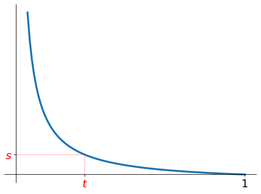
- In case 1, if \(\varphi(0+)=\infty\), then the properties from Definition 4.1 guarantee that \(\varphi: (0,1] \to [0,\infty)\) is bijective and hence we can just use the classic inverse. Cf. Figure 4.1 (a).
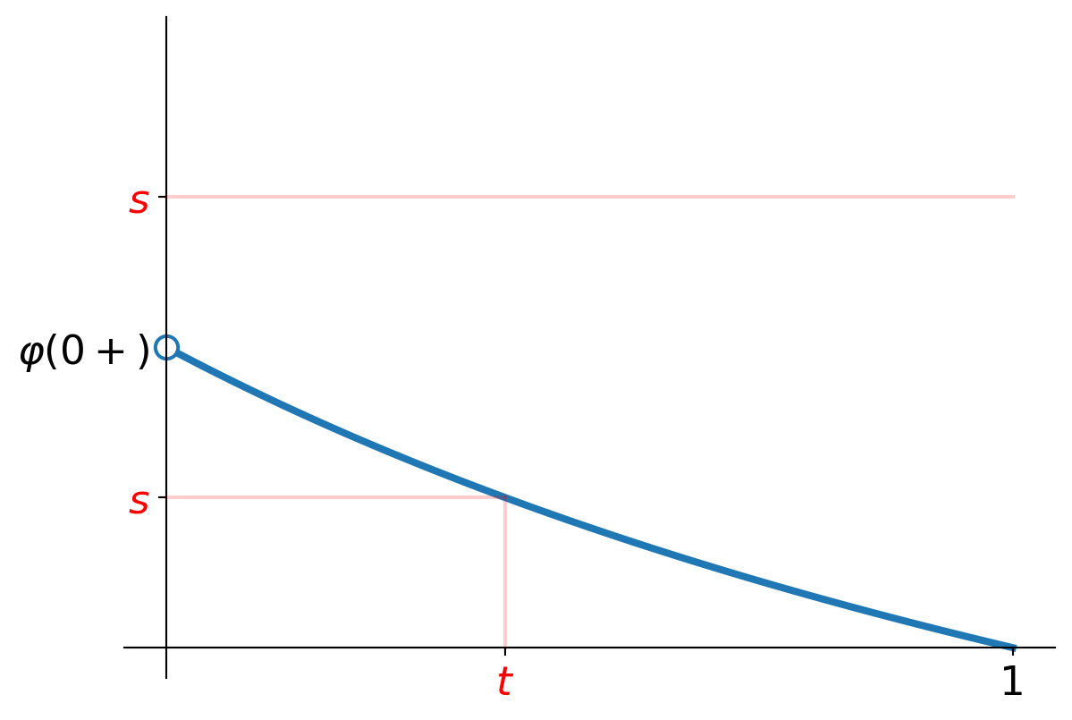
- In case 2, if \(\varphi(0+)<\infty\), again by the properties from Definition 4.1 \(\varphi\) is bijective as mapping from \((0,1]\) to \([0,\varphi(0+))\) and hence for any \(s \in [0,\varphi(0+))\) we can just use the classic inverse \(\varphi^{-1}(s)\). However for any \(s \geq \varphi(0+)\) the classic inverse is undefined. Cf. Figure 4.1 (b). It turns out, for the purposes of copula construction, that the value you want your inverse to take here is \(0\) so that’s the choice we make. Hence Equation 4.4. Note that one consequence of this choice is that it makes sure that \(\varphi^{[-1]}\) is continuous.
Example 4.2 Let’s work out the pseudo-inverse for the two examples of generators from Example 4.1.
For \(\varphi: (0,1] \to [0,\infty)\) given by \(\varphi(t)=-\log(t)\) we have that \(\varphi(0+)=\infty\), and hence the first case in Definition 4.2 kicks in: the pseudo-inverse is just the classic inverse, which you can readily work out. So the pseudo-inverse of this \(\varphi\) is the function \(\varphi^{[-1]}: [0,\infty) \to [0,1]\) given by \[\varphi^{[-1]}(s)=e^{-s} \quad \text{for all } s \in [0,\infty).\]
For \(\varphi: (0,1] \to [0,\infty)\) given by \(\varphi(t)=1-t\) we have that \(\varphi(0+)=1<\infty\), and hence we now need to use the second case in Definition 4.2. Since \(1-t=s\) yields \(t=1-s\) we can conclude that the pseudo-inverse of this \(\varphi\) is the function \(\varphi^{[-1]}: [0,\infty) \to [0,1]\) given by \[\varphi^{[-1]}(s)=\begin{cases} 1-s & \text{if } s \in [0,1) \\ 0 & \text{if } s \geq 1. \end{cases} \]
Here is then the big result for this section: how to construct a copula from a given Archimedean generator!
Theorem 4.1 Let \(\varphi\) be an Archimedean generator as defined in Definition 4.1, with pseudo-inverse \(\varphi^{[-1]}\) as defined in Definition 4.2. Then the mapping \(C: [0,1]^2 \to [0,1]\) defined by \[C(u,v)=\varphi^{[-1]} \big( \varphi(u)+\varphi(v) \big) \quad \text{for all } u,v \in (0,1) \tag{4.5}\] and with the usual values on the boundary of its domain (cf. Remark 3.1), is a copula. It is called the (Archimedean) copula generated by \(\varphi\).
We don’t discuss the proof, which (as you will have guessed) is essentially all technical work to show that this expression satisfies in particular condition iii of Definition 3.1. If you’re interested, see e.g. McNeil, Frey, and Embrechts (2015).
Now let’s go pick up some rewards for all our work here — we did all of this because it promised us a convenient way to construct examples of copula! Indeed we have already done part of the work for two examples of Archimedean generators in earlier examples, and let’s now apply the above result to see what copulas these generators yield:
Example 4.3 Consider the two generators from Example 4.1 again, for which we had already worked out the pseudo-inverses in Example 4.2. Now it is just a matter of plugging stuff into Equation 4.5 to get some copulas out!
For the generator \(\varphi: (0,1] \to [0,\infty)\) given by \(\varphi(t)=-\log(t)\) with pseudo-inverse given by \(\varphi^{[-1]}(s)=e^{-s}\), we get the following generated copula from Theorem 4.1. For any \(u, v \in (0,1)\) \[\begin{align*} C(u,v) &= \varphi^{[-1]} \big( \varphi(u)+\varphi(v) \big) \\ &= \varphi^{[-1]} \big( -\log(u)-\log(v) \big) \\ &= e^{-(-\log(u)-\log(v))} \\ &= e^{\log(u)+\log(v))} \\ &= e^{\log(u)} e^{\log(v)} \\ &= uv. \end{align*} \] Oi! That’s nothing but our friend from the very start: the independence copula we already encountered in Example 3.3, apparently that’s an Archimedean copula!
Next for the generator \(\varphi: (0,1] \to [0,\infty)\) given by \(\varphi(t)=1-t\). In Example 4.2 we had found its pseudo-inverse to be \[\varphi^{[-1]}(s)=\begin{cases} 1-s & \text{if } s \in [0,1) \\ 0 & \text{if } s \geq 1. \end{cases} \] So now we get the following from Theorem 4.1. For any \(u, v \in (0,1)\) \[\begin{align*} C(u,v) &= \varphi^{[-1]} \big( \varphi(u)+\varphi(v) \big) \\ &= \varphi^{[-1]} \big( (1-u)+(1-v) \big) \\ &= \varphi^{[-1]} \big( 2-u-v \big) \\ &= \begin{cases} 1-(2-u-v) & \text{if } 2-u-v \in [0,1) \\ 0 & \text{if } 2-u-v \geq 1 \end{cases} \\ &= \begin{cases} u+v-1 & \text{if } u+v-1 > 0 \\ 0 & \text{if } u+v-1 \leq 0 \end{cases} \\ &= \max\{u+v-1,0\}. \end{align*} \] Obviously, the last two steps are optional fiddling to get it into a nicer form — if you’re only after an expression for the copula (for instance in an assessment ;)) then it would be fine to stop after the fourth equality. Further note that in the fifth equality we used that \(2-u-v \in [0,1)\) is the same as \(2-u-v<1\) and hence \(u+v-1 > 0\), because we are working with \(u, v \in (0,1)\).
Well, isn’t this one big reunion party: this mystery guest is nothing but the countermonotonicity copula we got to know in Example 3.4!
Remark 4.2. Although Archimedean copulas form a very rich and convenient class and are commonly used for modelling etc. purposes, keep in mind that not every copula is Archimedean! Indeed as Equation 4.5 shows, any Archimedean copula \(C\) is symmetric in the sense that \(C(u,v)=C(v,u)\) for all \(u,v \in (0,1)\), but this is not generally true: there exist plenty of copulas that are not symmetric and hence definitely not Archimedean!
4.3 Some fiddling in R
Finally in this chapter, let’s look at doing some interesting stuff with copulas in R. There is a prominent R package called (indeed) copula (CRAN package page, documentation) that provides a wide range of functionality — for reasons of time and scope we’ll only look at a small part of it, but if you’re interested in further exploring it further then I can def recommend that!
Roughly speaking there is two categories of functionality:
- Given (the distribution of) a pair of random variables \((X,Y)\), do a variety of things with it, such as generating samples, evalute its joint cdf/pdf, compute any of a number of so-called measures of dependence that we’ll discuss in the next Chapter 5 etc.
- Given a set of data (in this context, points in \(\R^2\) that we assume to be samples/realisations of a pair of random variables \((X,Y)\) with unknown distribution), fit a distribution to that data.
In a general full workflow, you’d most likely use category 2 first to construct a specific model (i.e. a pair \((X,Y)\) with known distribution) fitting your past data (likely by working from a family of distributions/copulas as also mentioned in Section 4.1) and then use category 1 to draw relevant conclusions from your model to inform your risk management decisions. Although this is all quite fascinating, as mentioned previously in this course we’ll stay mostly away from the more Statsy side that is category 2 and look at category 1 only. And in particular, for the sake of time, we’ll in particular focus on generating samples as a tool to do some nice and insightful visual analysis as well as Monte Carlo style approximations. :).
4.3.1 What’s the use of generating samples?
The short answer: recall the plots we saw earlier in Example 3.2! The slightly more elaborate answer is as follows. Recall that a sample (or: realisation) from a pair \((X,Y)\) is a point \((x,y) \in \R^2\): imagine that we execute whatever experiment is hidden behind \((X,Y)\) once, so that \(X\) takes a value \(x \in \R\) and \(Y\) a value \(y \in \R\) or, equivalently, \((X,Y)\) takes the value \((x,y) \in \R^2\).
If we produce many samples, say \((x_1,y_1)\), \((x_2,y_2)\), …, \((x_n,y_n)\) and put them together in a scatterplot (as we did in Example 3.2), then this gives us a great visual impression of where in \(\R^2\) samples are more resp. less likely to end up. Recall from our Monte Carlo simulation discussions that in fact this visual impression is underpinned by/can be made more precise as follows: if we take any region \(B \subseteq \R^2\) and count the number of samples that ends up in that region, say \(r\), then \(r/n\) is a (good, if you use enough samples) approximation of the exact probability that \((X,Y)\) ends up in that region i.e. \(\P((X,Y) \in B)\). Mathematically (recall point 2 in Remark 1.1): \[\P((X,Y) \in B) \approx \frac{\text{Nr. of samples in } B}{n}. \tag{4.6}\]
Another powerful use is the approximation of the expectation of any real-valued function applied to \((X,Y)\), that is (cf. point 4 in Remark 1.1), for any \(g: \R^2 \to \R\) \[\E[g(X,Y)] \approx \frac{1}{n} \sum_{i=1}^n g(x_i,y_i). \tag{4.7}\]
Now, to connect up with earlier work, in some specific cases we could already generate samples from \((X,Y)\) and execute Equation 4.6 and/or Equation 4.7, namely:
- when \(X\) and \(Y\) are independent (seen in Example 3.2 and several exercises in Section 1.5 for instance),
- when the relationship between \(X\) and \(Y\) can be expressed in some direct functional way (like the pair \((X_2,Y_2)\) in Example 3.2 for instance).
What we add to that in this Section 4.3 is the ability to deal with a much wider range of interesting cases!
Remark 4.3. Also here keep our key visual Equation 3.9 firmly in mind: the distribution of a pair \((X,Y)\), and hence what a scatterplot of its samples looks like (as well as what values you get in the right hand side of Equation 4.6 and/or Equation 4.7), depends on all three of
- the marginal distribution of \(X\),
- the marginal distribution of \(Y\),
- the copula describing the dependency structure between \(X\) and \(Y\).
So if you change any of these three ingredients, then you should expect your scatter plot to change!
One aspect of this: the range of (the marginal distribution) of \(X\) (resp. the range of (the marginal distribution) of \(Y\)) determines the lower and upper limit of the \(x\)-values (resp. \(y\)-values) our samples can have. For instance, if the marginal distribution of \(X\) is \(\text{Unif}(0,1)\) then each sample \((x_i,y_i)\) will satisfy \(x_i \in (0,1)\) (because \((0,1)\) is the range of that distribution). Or if the marginal distribution of \(Y\) is \(\text{Exp}(1)\) then each sample \((x_i,y_i)\) will satisfy \(y_i \in (0,\infty)\). Or if \(X\) and \(Y\) each have a marginal Normal distribution, then a sample \((x_i,y_i)\) can very well pop up anywhere in \(\R^2\). (If you’re not sure how to find the range associated with a certain (continuous) distribution, then have a quick read of the discussion around Equation A.18.)
In general, if the range of \(X\) is an interval \((a,b)\) and the range of \(Y\) an interval \((c,d)\), then the rectangle in \(\R^2\) with lower left vertex/corner \((a,c)\) and upper right vertex/corner \((b,d)\) forms a “bounding box” for the samples: each sample \((x_i,y_i)\) will lie within this rectangle.
4.3.2 How to generate samples?
As mentioned at the start of Section 4.3 already, we’ll be using the copula package for this purpose. The good news is that the package has a number of well known (families of) copulas built-in ready to go. Combined with using only the built-in (real-valued) distributions in R (cf. Section 1.4.4) for our marginal distributons, generating samples from a pair is pretty starightforward. If you’re interested then it is definitely also possible to define “custom” copulas (or real-valued distributions) and get the copula package to work with those, but that requires more advanced R coding and I don’t think we should go there in this course.
After installing the copula package (which you have to do only once) and making it available in your session using the library(copula) command, you need (only) the following commands:
- Choose a copula you want to work with — for instance to create an R variable, say
cop, that contains/represents the Clayton copula with parameter \(\theta=3\) (recall from Section 4.1) usecop<-claytonCopula(param=3). - Use the
mvdc()function (doc) to create an R variable, saydistr, that contains/represents the distribution of a pair \((X,Y)\). The important (named) arguments of this function arecopula: the copula you want to use, in the form of an R variable (e.g.copfrom step 1),margins: a vector containing two strings, determining the marginal distributions of \(X\) and \(Y\) resp. — both these strings must be one of the built-in distribution names in R, cf. Section 1.4.4,paramMargins: a list with two entries, each entry a list/vector giving the parameters for the two marginal distributions you have chosen.
- Call the
rMvdc()function (doc) to generate samples. This function takes two (unnamed) arguments: the number of samples you want and the distribution you want to sample from (e.g. thedistrcreated in the previous step).
Putting that together in some concrete example code looks like Listing 4.1 below. We use a pair \((X,Y)\) specified by the marginal distributions \(X \sim \mathcal{N}(0,1)\) and \(Y \sim \text{Exp}(1)\), plus the Clayton copula (cf. Equation 4.1) with \(\theta=3\).
Recall from Remark 4.3 that this means that a sample \((x,y)\) from \((X,Y)\) has the property that \(y \in (0,\infty)\) while \(x\) can be anywhere on the real line (in principle, but is most likely to be somewhere not too far from \(0\)). Check for yourself that this is indeed the case for all points in the scatterplot in below output.
Further note that for the approximation of \(\E[X^2 \cos(Y)]\) we do in the below code (because why not) we use Equation 4.7, as well as the mapply route we also used in Exercise 1.3 e.g.
Remark 4.4. Are you ready for a brain twister?? Ok here goes. Suppose that in the code Listing 4.1 above we would change the parameter value of the copula to some other value than \(3\) and run it again. Which bits of output would change? Well we change the copula, and hence the distribution of the pair \((X,Y)\) (recall Remark 4.3!), and hence all the output would change no?
Yes very good! But also not entirely ;). The QQ-plots will not change (much), these will still show a pretty much perfect fit to these same red lines — after all, we don’t change the marginal distributions of \(X\) and \(Y\).
So hang on. If we compare two runs of this code, one with \(\theta=3\) and one with \(\theta=10\) say, then if we focus on the samples of \(X\) only we get two essentially interchangable sets of values. And the same for the samples of \(Y\). But how is that possible, while at the same time it is also true that the samples of \((X,Y)\) are definitely not interchangeable between these runs???
Here’s the answer. Suppose that I tell you that I have two points in \(\R^2\), with \(x\)-coordinates say \(1\) and \(2\) and \(y\)-coordinates say \(3\) and \(4\). Do you then know for sure which points I’m taking about? No! I could be talking about the points \((1,3)\) and \((2,4)\), but also about the points \((1,4)\) and \((2,3)\). So: to specify a set of points in \(\R^2\) it is not enough to only know the \(x\)-coordinates and the \(y\)-coordinates, we also need to know which \(x\)-coordinate gets paired up with which \(y\)-coordinate exactly! As you’ll easily be able to imagine, if we have a large \(n\) number of \(x\) and \(y\)-coordinates, then different choices for how we pair these up can result in wildly different sets of points in \(\R^2\).
This gives us another manifestation of our queen of all visuals Equation 3.9, if we think about it from the perspective of a scatterplot filled with samples of \((X,Y)\) (points in \(\R^2\)):
- the \(x\)-coordinates of these points are samples from \(X\) and hence only depend on the marginal distribution of \(X\),
- the \(y\)-coordinates of these points are samples from \(Y\) and hence only depend on the marginal distribution of \(Y\),
- the dependency structure/copula determines how these \(x\) and \(y\)-coordinates are exactly paired up to form the points in \(\R^2\) and hence the scatterplot we ultimately get to see.
Note how this also nicely ties in with an intuitive understanding of what dependence is, namely that it is about certain samples of \(X\) and \(Y\) being more likely to appear together and others less likely to appear together.
4.3.3 Visualising the Clayton family
Let’s now do some more systematic exploration of the Clayton family of copulas from Section 4.1, by taking a pair of random variables \((X,Y)\) with both a marginal \(\text{Unif}(0,1)\) distribution (so that all samples are contained in the unit square \((0,1)^2\) in \(\R^2\), cf. Remark 4.3) and with the Clayton copula. By walking through a sequence of different parameter values \(\theta\) in the parameter space \([-1,0) \cup (0,\infty)\) (cf. Equation 4.1) and creating a scatterplot of samples from \((X,Y)\) at each step, we can visually inspect the scatterplot pattern generated by these different parameter choices. Keep in mind that since we keep the marginal distributions constant, any changes we see from one step to the next are solely due to the change in the copula!
There is a lot of interesting stuff to see in the output of the above Listing 4.2!
Note that if we plug \(\theta=-1\) into Equation 4.1 then the resulting copula is \[C_{-1}(u,v)=\max\{u+v-1,0\} \quad \text{for all } u,v \in (0,1),\] which is a very familiarly looking one: indeed it is the countermonotonicity copula we previously already encountered in Example 3.4 and Exercise 3.4! Recall from Exercise 3.4 that this copula represents “full negative” dependence: there exists a decreasing function \(f: \R \to \R\) so that \(Y=f(X)\). It doesn’t specify what function \(f\) this exactly is, in fact that depends on the marginal distributions that have been chosen. In this case, with \(\text{Unif}(0,1)\) marginals, it is the function \(f(x)=1-x\) (as already seen in Example 3.2).
So, in conclusion: if we choose \(\theta=-1\) then we enforce that our pair \((X,Y)\) satisfies the relationship \(Y=1-X\). And hence a set of samples \((x_1,y_1)\), …, \((x_n,y_n)\) would all have the property that \(y_i=1-x_i\) i.e. all these samples/points lie on the graph of the function \(f(x)=1-x\) for \(x \in (0,1)\). Indeed we have already seen exactly that scatterplot in Example 3.2!
Now move on to the first scatterplot in the output above, for \(\theta=-0.9\). Generally scatterplots will change “smoothly” with small changes in copula parameter values2. Indeed if we take the picture we described in the above bullet point for \(\theta=-1\) and compare it with this one for \(\theta=-0.9\), we see that there are still a lot of samples located very closely to the graph of \(f(x)=1-x\) — though we see they are “sagging” a bit further towards the origin, and there is a scattering of more adventurous ones throughout the top right region of the unit square.
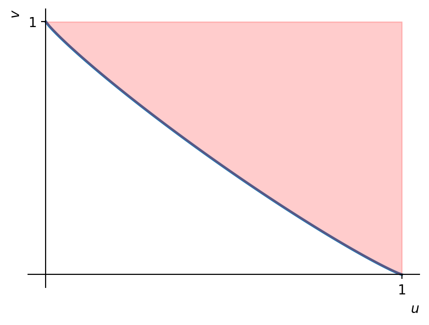
One thing that rather stands out: all samples are only on top or above that “sagging line”, none are below it! Is that a coincidence? It could be — after all there is always the reservation that a scatterplot only gives an approximate picture of the true distribution of \((X,Y)\) (due to the fact that we use only finitely many samples, the fundamental weakness of any sampling/Monte Carlo based approach as also discussed in Remark 1.2) — yet it would be a very unlikely coincidence… Indeed it isn’t a coincidence and in fact we can see this behaviour “encoded” in our copula! If we plug \(\theta=-0.9\) into Equation 4.1 then we get the expression \[C_{-0.9}(u,v)=\left( \max\{u^{0.9}+v^{0.9}-1,0\} \right)^{10/9} \quad \text{for all } u,v \in (0,1),\] i.e. \(C_{-0.9}(u,v)\) equals \((u^{0.9}+v^{0.9}-1)^{10/9}\) if \(u^{0.9}+v^{0.9}-1>0\) and it equals \(0\) otherwise. If we visualise this then we get Figure 4.2: we see the domain of \(C_{-0.9}\), namely the unit square in the \(u\)-\(v\)-space, the blue curve all \((u,v)\) that satisfy \(u^{0.9}+v^{0.9}-1=0\), and in red the region in that space containing all \((u,v)\) with \(u^{0.9}+v^{0.9}-1>0\). So in particular, the white region below the blue curve are all \((u,v)\) with \(u^{0.9}+v^{0.9}-1<0\) and hence \(C_{-0.9}(u,v)=0\). (Note also how this blue curve seems to coincide remarkably well with the “sagging line” in the output of Listing 4.2 for \(\theta=-0.9\)…). And these observations are in fact sufficient to confirm that it is indeed (essentially) impossible for any sample of \((X,Y)\) to end up below that “sagging line”! Cf. Exercise 4.4 (wouldn’t want to keep all the fun to myself! ;)).
2 Provided the copula depends in a smooth way, say continuously, on the parameter
Next if we consider the scatterplots as \(\theta\) further grows through the interval \([-1,0)\) up until \(\theta=-0.1\), then we see that the points ever further spread out: we “sag” ever further towards the origin, and they also get less concentrated around the “sagging line”. For \(\theta=-0.1\) we see hardly any pattern at all anymore, it seems like a pretty much arbitrary scattering of points through the unit square \((0,1)^2\). That might already make you think of independence, and if not yet then compare with the scatterplot for the independent case we made earlier in Example 3.2 — very similar indeed!
So this suggests that as \(\theta \uparrow 0\), we get ever closer to independence. As you’ll remember, we know quite well what copula represents independence, our eternal friend the independence copula \((u,v) \mapsto uv\) (recall from Example 3.3 e.g.). So on this basis we have the strong suspicion that it holds for any \(u,v \in (0,1)\) that \[\begin{align*} \lim_{\theta \uparrow 0} C_\theta(u,v) &= \lim_{\theta \uparrow 0} C_\theta(u,v) \\ &= \lim_{\theta \uparrow 0} \left( \max\{u^{-\theta}+v^{-\theta}-1,0\} \right)^{-1/\theta} \\ &= uv \end{align*} \] Indeed it turns out that this convergence is actually not that difficult to prove (take the logarithm of \(C_\theta(u,v)\), then apply l’Hoptial’s rule and a bit of algebra — don’t worry about the details obviously). There is a cute alternative way to see this: the Clayton family is Archimedean with generator \[\varphi_\theta(t)=\frac{1}{\theta}\left( t^{-\theta}-1 \right),\] and if we let \(\theta \uparrow 0\) the limit is \(t \mapsto -\log(t)\), exactly the generator of the independence copula as we saw in Example 4.3!
Finally then, if we let \(\theta\) grow beyond \(0\) to larger values then we see that we gradually move away from the arbitrary scattering resulting from independence towards a new interesting shape: an ever more pronounced clustering of the samples on the diagonal! In the language of Remark 4.4 (another use of that language in Exercise 4.4): as \(\theta\) grows the “matching mechanism” that is the copula has an ever stronger tendency to match small samples of \(X\) with small samples of \(Y\), and to match large samples of \(X\) with large samples of \(Y\). If we imagine this pattern persisting for values for \(\theta\) beyond \(150\), then we would expect that in the limit \(\theta \to \infty\), all samples end up exactly on the diagonal i.e. that all samples \((x_i,y_i)\) satisfy \(x_i=y_i\). That is to say, that in limit we end up with the relationship \(Y=X\). This is another special case, namely “full positive dependence” if you will, that we earlier discussed in Exercise 3.4, and is represented by the comonotonicity copula \((u,v) \mapsto \min\{u,v\}\).
Indeed, similar as in point 3 above, we can make this visual inspiration precise: it can be shown that \[\begin{align*} \lim_{\theta \to \infty} C_\theta(u,v) &= \lim_{\theta \to \infty} C_\theta(u,v) \\ &= \lim_{\theta \to \infty} \left( \max\{u^{-\theta}+v^{-\theta}-1,0\} \right)^{-1/\theta} \\ &= \min\{u,v\}. \end{align*} \]
4.4 Some exercises
NoteAbout the exercises
Each exercise has a (rough) indication of its difficulty, as follows:
| * | easier: can be solved by (almost) only using relevant definitions/results, |
| ** | medium: in addition to relevant definitions/results, needs a limited amount of work/creativity, |
| *** | harder: in addition to relevant definitions/results, needs a larger amount of work/serious creativity, |
| 💀 | warning: might make your brain hurt! These are mainly intended to provide some extra challenge for those of you keen on that and are generally quite hard. You don't need to worry about these too much for exam purposes. |
The exam consists of mostly ** and *** level questions, some *, and possibly at most a few marks worth of 💀.
A bit of preaching: it is an incredibly important part of the study process to try and work on the exercises as much as possible. To become a better mathematician/learn new maths (and also to get a good exam mark ;)), above all you need to do it. And yes, of course that includes falling over things, and making mistakes, and getting stuck, and getting frustrated — all part of the game and what you’re supposed to be doing! Your lecturers have done that as well and still do it. What matters is that you don’t let that discourage you and that you make good use of the help and resources available to help you develop your skills. As part of that, many exercises have a hint in a block like this:
NoteHint (click to view)
Hint!
These are trying to help you on your way if you don’t know where to start or to provide some ideas if you get stuck. In spirit of the above, always have a look at these first and try again before you look at the full solution. (These hints are an extra service that won’t be available in the exam I’m afraid ;).)
Of course, we have our classes and there’s office hours, email etc. as well — I’m at any time very happy to help you with any questions you may have, and you should please never feel that any question is “too dumb” to ask!
Full/detailed solutions for the exercises will become available, just immediately below the exercises, immediately after our tutorial hour (you may have to refresh the page).
Exercise 4.1 [**] Consider the mapping \(\varphi_\theta: (0,1] \to [0,\infty)\) given by \[\varphi_\theta(t)=e^{\theta/t}-e^\theta \quad \text{for all } t \in (0,1],\] where \(\theta \in (0,\infty)\) is a parameter.
- Show that \(\varphi_\theta\) is an Archimedean generator.
- Find an expression for the copula generated by \(\varphi_\theta\).
NoteHint (click to view)
Part i is a matter of checking the conditions from Definition 4.1, and part ii needs an application of Theorem 4.1, if you need some inspiration then review Example 4.2 & Example 4.3!
TipFull solution (click to view)
For part i, we need to check the four conditions listed in Definition 4.1:
- The continuity is clear since it’s a composition of elementary functions that we know well to be continuous.
- We have for any \(t \in (0,1)\) that \[\varphi_\theta'(t)=-\theta t^{-2} e^{\theta/t}<0.\]
- For any \(t \in (0,1)\) we have that \[\varphi_\theta''(t)=2\theta t^{-3} e^{\theta/t}+\theta^2 t^{-4} e^{\theta/t} \geq 0.\]
- Clearly \[\varphi_\theta(1)=e^\theta-e^\theta=0.\]
For part ii, this is matter of applying Theorem 4.1: the copula \(C_\theta\) (for clarity we attach a \(\theta\) here as well, to indicate its dependence on the parameter, but obviously that’s a bit of sugar coating the notation only that’s otherwise not important) generated by \(\varphi_\theta\) is given by \[C_\theta(u,v)=\varphi_\theta^{[-1]} \big( \varphi_\theta(u)+\varphi_\theta(v) \big) \quad \text{for all } u,v \in (0,1). \tag{4.8}\] So it’s the same two-step process as in Example 4.2 & Example 4.3: first determine the pseudo-inverse \(\varphi_\theta^{[-1]}\), and then work out Equation 4.8.
For the pseudo-inverse, recall from Definition 4.2 and Example 4.2 that we first need to see which of the two possible cases we’re dealing with here: \(\varphi_\theta(0+)=\infty\) or \(\varphi_\theta(0+)<\infty\). Clearly \[\varphi_\theta(0+)=\lim_{t \downarrow 0} \varphi_\theta(t)=\lim_{t \downarrow 0} e^{\theta/t}-e^\theta = e^{\infty}-e^\theta=\infty,\] and hence the pseudo-inverse \(\varphi_\theta^{[-1]}: [0,\infty) \to [0,1]\) is just the classic inverse: for any \(s \in [0,\infty)\) we have that \[\varphi_\theta(t)=s \iff e^{\theta/t}-e^\theta=s \iff t=\frac{\theta}{\log(s+e^\theta)}.\] So \(\varphi_\theta^{[-1]}: [0,\infty) \to [0,1]\) is given by \[\varphi_\theta^{[-1]}(s)=\frac{\theta}{\log(s+e^\theta)} \quad \text{for all } s \in [0,\infty).\]
Now we have everything we need to work out Equation 4.8: for any \(u,v \in (0,1)\) \[\begin{align*} C_\theta(u,v) &= \varphi_\theta^{[-1]} \big( \varphi_\theta(u)+\varphi_\theta(v) \big) \\ &= \varphi_\theta^{[-1]} \left( e^{\theta/u}-e^\theta+e^{\theta/v}-e^\theta \right) \\ &= \frac{\theta}{\log \left( e^{\theta/u}-e^\theta+e^{\theta/v}-e^\theta+e^\theta \right)} \\ &= \frac{\theta}{\log \left( e^{\theta/u}+e^{\theta/v}-e^\theta \right)}. \end{align*} \]
Exercise 4.2 [**] Let the function \(\varphi: (0,1] \to [0,\infty)\) be given by \[\varphi(t)=-\log \left( \frac{t+1}{2} \right) \quad \text{for all } t \in (0,1].\]
- Show that \(\varphi\) is an Archimedean generator.
- Show that the copula generated by \(\varphi\) is given by \[C(u,v)=\max \left\{ \frac{1}{2} (u+1)(v+1) -1,0 \right\} \quad \text{for all } u,v \in (0,1).\]
NoteHint (click to view)
Follow exactly the same ideas as in Exercise 4.1. For part ii, after you’ve worked out the expression for the copula from Theorem 4.1 it initially won’t look anything like the expression for \(C\) we’re trying to show, but then throwing some basic algebra at that expression will get you there!
TipFull solution (click to view)
For part i, again we need to check the four conditions listed in Definition 4.1:
- The continuity is clear since it’s a composition of elementary functions that we know well to be continuous.
- We have for any \(t \in (0,1)\) that \[\varphi'(t)=-\frac{1}{t+1}<0.\]
- For any \(t \in (0,1)\) we have that \[\varphi_\theta''(t)=\frac{1}{(t+1)^2} \geq 0.\]
- Clearly \[\varphi_\theta(1)=-\log(1)=0.\]
For part ii, we follow the same strategy as in part ii of Exercise 4.1: we first determine the pseudo-inverse using Definition 4.2 and then apply Theorem 4.1.
For the pseudo-inverse, we start by determining which of the two cases we’re in: \[\varphi(0+)=\lim_{t \downarrow 0} \varphi(t)=\lim_{t \downarrow 0} -\log \left( \frac{t+1}{2} \right) = -\log \left( \frac{1}{2} \right)<\infty\] (don’t get confused: since \(\log(1/2)<0\), \(\varphi(0+)\) is positive as it should be!). So we get from Definition 4.2 that the pseudo-inverse \(\varphi^{[-1]}: [0,\infty) \to [0,1]\) is given by \[\varphi^{[-1]}(s)=\begin{cases} \varphi^{-1}(s) & \text{if } s \in [0,-\log(1/2)) \\ 0 & \text{if } s \geq -\log(1/2), \end{cases} \tag{4.9}\] where \(\varphi^{-1}\) is the classic inverse that we determine in the usual way: for any \(s \in [0,-\log(1/2))\) \[s=\varphi(t) \iff s=- \log \left( \frac{t+1}{2} \right) \iff t=2e^{-s}-1,\] so \(\varphi^{-1}(s)=2e^{-s}-1\). Plugging this back into Equation 4.9 results in the final expression for the pseudo-inverse: \[\varphi^{[-1]}(s)=\begin{cases} 2e^{-s}-1 & \text{if } s \in [0,-\log(1/2)) \\ 0 & \text{if } s \geq -\log(1/2). \end{cases} \]
Now we are read to work out the copula by appealing to Theorem 4.1: for any \(u,v \in (0,1)\) we get \[\begin{align*} C(u,v) &= \varphi^{[-1]} \big( \varphi(u)+\varphi(v) \big) \\ &= \varphi^{[-1]} \left( -\log \left( \frac{u+1}{2} \right) -\log \left( \frac{v+1}{2} \right) \right) \\ &= \begin{cases} 2 e^{\big( \log((u+1)/2)+\log((v+1)/2) \big)}-1 & \text{if } -\log((u+1)/2)-\log((v+1)/2) \in [0,-\log(1/2)) \\ 0 & \text{if } -\log((u+1)/2)-\log((v+1)/2) \geq -\log(1/2). \end{cases} \end{align*} \] Now, in principle this expression is enough: as soon as we have an expression for the copula in terms of \(u\) and \(v\) only (i.e. not any further presence of \(\varphi\) and/or \(\varphi^{[-1]}\)) then we have achieved our essential goal. However in this question we are asked to go slightly further, and to simplify the above expression for \(C\) to the one given in the question.
For this, first note that by the usual rules for working with logs, we can write \[\log \left( \frac{u+1}{2} \right)+\log \left( \frac{v+1}{2} \right)=\log \left( \frac{(u+1)(v+1)}{4} \right)\] so that we can simplify to \[C(u,v) = \begin{cases} \frac{1}{2} (u+1)(v+1) -1 & \text{if } -\log((u+1)(v+1)/4) \in [0,-\log(1/2)) \\ 0 & \text{if } -\log((u+1)(v+1)/4) \geq -\log(1/2). \end{cases}\] Further note that since \(u,v \in (0,1)\) we have in particular that \(u+1<2\) and \(v+1<2\) so that \((u+1)(v+1)/4<1\) and hence \(-\log((u+1)(v+1)/4)>0\). So \[-\log((u+1)(v+1)/4) \in [0,-\log(1/2)) \iff -\log((u+1)(v+1)/4)<-\log(1/2)\] which can easily be further rewritten to \((u+1)(v+1)>2\) and hence to \((u+1)(v+1)/2-1>0\). This allows us to further simplify the above expression to \[C(u,v) = \begin{cases} \frac{1}{2} (u+1)(v+1) -1 & \text{if } \frac{1}{2} (u+1)(v+1) -1>0 \\ 0 & \text{if } \frac{1}{2} (u+1)(v+1) -1 \leq 0. \end{cases}\] And this is, of course, exactly the same as \[C(u,v)=\max \left\{ \frac{1}{2} (u+1)(v+1) -1,0 \right\}\] so we’re finally there! :).
Exercise 4.3 [***] Let \(\varphi: (0,1] \to [0,\infty)\) be the Archimedean generator of a copula \(C\). Assume for simplicty that \(\varphi\) is twice differentiable on \((0,1)\) and that \(\varphi(0+)=\infty\). For a parameter \(\theta \in (0,\infty)\), define the function \(\varphi_\theta: (0,1] \to [0,\infty)\) as \[\varphi_\theta(t)=\theta \cdot \varphi(t) \quad \text{for all } t \in (0,1].\]
- Show that \(\varphi_\theta\) is also an Archimedean generator.
- For any \(\theta \in (0,\infty)\), let \(C_\theta\) be the copula generated by \(\varphi_\theta\). Find out how \(C_\theta\) relates to \(C\).
NoteHint (click to view)
For part i, we’ll need to check that the four points in Definition 4.1 hold as we did in the previous exercises as well. However because we now have only an implicit expression, it requires maybe a bit more thinking. Obviously make optimal use of the information about \(\varphi\) that we have, and make (careful) use of the “notes” listed in Definition 4.1!
For part ii, we’ll have to use Theorem 4.1 to obtain expressions for the copulas involved. The obstacle to then comparing them is the presence of these pseudo-inverses in these expressions. To deal with this, make the observation that the pseudo-inverses simplify to classic inverses in this case, and establish a relationship between these. If you get stuck at this point, then the relationship you’re looking to prove is that \[\varphi_\theta^{-1}(s)=\varphi^{-1} \left( \frac{s}{\theta} \right) \quad \text{for all } s \in [0,\infty).\] You should ultimately find that the copula generated by \(\varphi_\theta\) is in fact identical to the one generated by \(\varphi\)!
TipFull solution (click to view)
For part i, again it’s all about the four conditions listed in Definition 4.1 — though we have to be slightly careful to use the correct logic!
- Multiplying a continuous function by a constant obviously again yields a continuous function.
- For any \(0 <t_1<t_2 \leq 1\) we have that \[\varphi_\theta(t_2)-\varphi_\theta(t_1)=\theta \varphi(t_2)-\theta \varphi(t_1)=\theta \big( \varphi(t_2)-\varphi(t_1) \big).\] Since \(\varphi\) is a generator it is strictly decreasing, i.e. \(\varphi(t_2)-\varphi(t_1)<0\). So also \(\varphi_\theta(t_2)-\varphi_\theta(t_1)<0\).
- As noted in Definition 4.1, for twice differentiable functions, convexity is equivalent to the second derivative being non-negative on \((0,1)\). Since \(\varphi\) is a twice differentiable generator, \(\varphi_\theta\) is also twice differentiable with \[\varphi_\theta''(t)=\theta \varphi''(t) \geq 0 \quad \text{for all } t \in (0,1).\]
- Clearly
\[\varphi_\theta(1)=\theta \varphi(1)=0.\]
Note: you may wonder why in point 2 we didn’t go via the first derivative. It’s a bit subtle, but the point is that strictly decreasing is not equivalent to the first derivative being strictly negative: obviously this is a sufficient condition but not a necessary one! So the fact that \(\varphi_\theta\) is a generator does not (necessarily) imply that \(\varphi_\theta'<0\) on \((0,1)\).
For part ii, all we have to get a handle on the copulas is Theorem 4.1, so we’ll again need to use it. It tells us that \[C(u,v) = \varphi^{[-1]} \big( \varphi(u)+\varphi(v) \big) \quad \text{for all } u,v \in (0,1) \tag{4.10}\] and \[\begin{align*} C_\theta(u,v) &= \varphi_\theta^{[-1]} \big( \varphi_\theta(u)+\varphi_\theta(v) \big) \\ &= \varphi_\theta^{[-1]} \big( \theta \varphi(u)+ \theta \varphi(v) \big) \quad \text{for all } u,v \in (0,1). \end{align*} \tag{4.11}\] As things stand, we can’t really compare these two expressions in a sensible way since we don’t know how \(\varphi_\theta^{[-1]}\) compares to \(\varphi^{[-1]}\). So let’s figure this out!
We’re given that \(\varphi(0+)=\infty\) and hence also \[\begin{align*} \varphi_\theta(0+) &= \lim_{t \downarrow 0} \varphi_\theta(t) \\ &= \lim_{t \downarrow 0} \theta \varphi(t) \\ &= \theta \lim_{t \downarrow 0} \varphi(t) \\ &= \theta \varphi(0+) \\ &= \infty, \end{align*} \] so Definition 4.2 tells us that both the pseudo-inverses \(\varphi^{[-1]}: [0,\infty) \to [0,1]\) and \(\varphi_\theta^{[-1]}: [0,\infty) \to [0,1]\) simplify to just the classic inverses \(\varphi^{-1}: [0,\infty) \to [0,1]\) and \(\varphi_\theta^{-1}: [0,\infty) \to [0,1]\). We can relate these for instance as follows, for any \(s \in [0,\infty)\) we can just work out the inverse of \(\varphi_\theta\) in the usual way: \[\varphi_\theta(t)=s \iff \theta \varphi(t)=s \iff \varphi(t)=\frac{s}{\theta} \iff t=\varphi^{-1} \left( \frac{s}{\theta} \right)\] (note that in the final step we used that \(\varphi\) has a classic inverse, so we don’t need to worry about the subtleties of generalised inverses etc. that we encountered previously!) so \[\varphi_\theta^{[-1]}(s)=\varphi_\theta^{-1}(s)=\varphi^{-1} \left( \frac{s}{\theta} \right) \quad \text{for all } s \in [0,\infty). \tag{4.12}\]
With this established, we can now go back to the above expressions for the copulas: for any \(u,v \in (0,1)\) fixed, Equation 4.10 becomes \[C(u,v) = \varphi^{-1} \big( \varphi(u)+\varphi(v) \big) \tag{4.13}\] while Equation 4.11 becomes \[\begin{align*} C_\theta(u,v) &= \varphi_\theta^{[-1]} \big( \theta \varphi(u)+ \theta \varphi(v) \big) \\ &= \varphi^{-1} \left( \frac{\theta \varphi(u)+ \theta \varphi(v)}{\theta} \right) \\ &= \varphi^{-1} \big( \varphi(u)+\varphi(v) \big) \\ &= C(u,v), \end{align*} \] where the second equality uses Equation 4.12 and the final one uses Equation 4.13.
So, interestingly, the conclusion is that if we multiply a generator by a positive constant to construct a new one, then this somehow does not change the copula it generates!
Exercise 4.4 [***] In this question (which is not very easy for many of you I’d guess, but it can really help you build your understanding so do try to have a go/review!) we revisit point 2 in Section 4.3.3, where we discussed the scatterplot we got for a pair \((X,Y)\) with marginal \(\text{Unif}(0,1)\) distributions and as copula the Clayton one with parameter \(\theta=-0.9\). Have another read of the discussion there and then have a go at the below questions.
- Complete the conclusion there by proving the following: for any \(x,y \in (0,1)\) satisfying \(x^{0.9}+y^{0.9}-1 \leq 0\) we have that \(\P(X \leq x \ \& \ Y \leq y)=0\), and explain how this confirms that we should indeed not expect to see any samples of \((X,Y)\) below the “sagging line” in the scatterplot for \(\theta=-0.9\) as produced by Listing 4.2.
- Play a bit around with scatterplots for different pairs \((X,Y)\) as produced in Listing 4.2, where you keep the copula the same (still the Clayton one with parameter \(\theta=-0.9\)) but change the marginal distributions to some other choices to your liking (best to stay with continuous distributions though). Is the “sagging line” we brought up in part i still present? If so, in what shape? Can you identify a common theme, maybe in terms of the language we used in Remark 4.4 to express what the role of a copula is?
NoteHint (click to view)
For part i, in very brief the chain of arguments is: \[\P(X \leq x \ \& \ Y \leq y)=F_{X,Y}(x,y)=C_{-0.9} \left( F_X(x),F_Y(y) \right)=C_{-0.9} (x,y)=0.\] Now you go justify each of these equalities!
For part ii, recall that Remark 4.4 contains the phrase “the dependency structure/copula determines how these \(x\) and \(y\)-coordinates are exactly paired up to form the points in \(\R^2\) and hence the scatterplot we ultimately get to see.”. If you look at the empty region below the “sagging line” in the scatterplot produced in Listing 4.2 for \(\theta=-0.9\), what does that tell about the “pairing up” referred to in that phrase, and how does that manifest itself in the other scatterplots you’re asked to make in this part ii?
TipFull solution (click to view)
For part i, fix any \(x,y \in (0,1)\) satisfying \(x^{0.9}+y^{0.9}-1 \leq 0\). We’re asked to compute a probability for our pair \((X,Y)\) i.e. we need to do something with its joint cdf \(F_{X,Y}\). In fact, by very def (cf. Equation A.25) of course the probability we’re asked to compute is exactly equal to the cdf evaluted in the \(x,y\) we have fixed: \[\P(X \leq x \ \& \ Y \leq y)=F_{X,Y}(x,y). \tag{4.14}\]
Now, in light of our key visual Equation 3.9: we know all ingredients on the ultimate right (the marginal distributions as well as the copula) and so we should be able to derive the joint cdf. Indeed, as always in this situation, Sklar’s theorem (cf. Theorem 3.1) to the rescue: it tells us that \[F_{X,Y}(x,y)=C_{-0.9} \left( F_X(x),F_Y(y) \right).\] Further, since \(x,y \in (0,1)\) and the marginal distributions of \(X\) and \(Y\) are \(\text{Unif}(0,1)\), we know quite well that \(F_X(x)=x\) and \(F_Y(y)=y\) (cf. Equation 2.2 e.g.) so that we in fact have that \[F_{X,Y}(x,y)=C_{-0.9} \left( x,y \right).\] Now review Figure 4.2: since the \(x,y\) we have fixed satisfy \(x^{0.9}+y^{0.9}-1 \leq 0\), the point \((x,y)\) is in that plot located either on the blue curve, or below it in the white region. As discussed above that plot, that means that \(C_{-0.9} (x,y)=0\). Hence \(F_{X,Y}(x,y)=0\) and plugging this back into Equation 4.14 we indeed arrive at \[\P(X \leq x \ \& \ Y \leq y)=0\] as we wanted!
Next for the second question in part i, to explain how this confirms that we should indeed not expect to see any samples of \((X,Y)\) below the “sagging line” in the scatterplot of \((X,Y)\) for \(\theta=-0.9\) as produced by Listing 4.2. If we fix any point \((x,y)\) in that scatterplot below that “sagging line” then (using on the visual observation that this “sagging line” is in the same location as the blue curve is in Figure 4.2) then the above shows that we have that \(\P(X \leq x \ \& \ Y \leq y)=0\) i.e. that the probability that \((X,Y)\) ends up in/generates a sample in the rectangle with lower left vertex the origin and upper right vertex the point \((x,y)\), is \(0\). So indeed you won’t find any samples at all in that rectangle! And since this argument applies to any point \((x,y)\) below that “sagging line”, indeed we won’t find any samples at all anywhere below that “sagging line”!
For part ii, obviously it is up to you what marginals you choose — I’d really encourage you to try several as it’s very insightful! Below in Listing 4.4 what things would look like if we switch to standard Normal marginals and to a combination of Exponential and Gamma marginals.
Is the “sagging line” still there? Well yes, quite clearly in both plots — in the first one it becomes even a seemingly straight line, while in the second it has a much more curved shape than the one in Listing 4.2. If we compare/contrast the plots, then we see clear differences but also a clear common theme: there is always some curve/“sagging line” that splits the picture in two parts: a “top right” part where all the samples are (mostly concentrated near the curve) and a “lower left” part where there are no samples at all. Let’s interpret this in the formulation of Remark 4.4.
Why do we see differences? Well because we are changing the marginal distributions, and as pointed out in Remark 4.4: this means that we get fundamentally different samples from \(X\) and/or \(Y\) (depending on which marginal distribution(s) we change). You can see this also manifested if you look at the scales on the horizontal and vertical axes and how these change between the different plots.
Why do we see a common theme? Well because we are keeping our copula the same, and hence, per Remark 4.4, how the pairing up of samples from \(X\) with samples of \(Y\) is done. If we look at the original scatterplot in Listing 4.2, then we can think about the empty “lower left” part of that plot as follows: apparently the copula ensures that smaller samples of \(X\) (keeping in mind the marginals are there \(\text{Unif}(0,1)\), so smaller there means closer to \(0\) than to \(1\)) get paired up with larger samples \(Y\) (also marginally \(\text{Unif}(0,1)\), so that means closer to \(1\) than to \(0\)). Indeed that effect leaves the “lower left” part empty, because any points in that part have small \(x\) and \(y\)-coordinates.
And we see that, because we keep the copula the same and hence this same matching mechanism in tact, that same “empty lower left” part popping up in the scatterplots we made below as well (plus any you made yourself). What the shape/location of that “empty lower left” exactly is depends on what “small values” and “large values” exactly mean for the marginal distributions at hand and so will change from one scatterplot to the next.
If you get to this point and think “damn that’s all quite subtle and hard to fully get my finger behind!” then yes, I can definitely imagine! To grow a better understanding and in particular stronger intuition for this stuff is above all a matter of time and working a lot with it, to make arguments like the above (and even more subtle ones) ever more clear and automatic for you. Obviously it wouldn’t be a reasonable expectation that you manage to develop all of that in a few weeks of talking about this stuff, while also battling your other courses etc. So don’t worry about that — if the above makes some sense to you then it’s mission accomplished and you have a good base to further develop your understanding & intuition from should you encounter copulas again at some later point in your career for instance!