\[ \renewcommand{\P}{\mathop{\mathbb{P}}\nolimits} \newcommand{\E}{\mathop{\mathbb{E}}\nolimits} \newcommand{\var}{\mathop{\rm Var}\nolimits} \newcommand{\VaR}{\mathop{\rm VaR}\nolimits} \newcommand{\cte}{\mathop{\rm CTE}\nolimits} \newcommand{\cov}{\mathop{\rm Cov}\nolimits} \newcommand{\limsup}{\mathop{\rm limsup}} \newcommand{\liminf}{\mathop{\rm liminf}} \newcommand{\R}{\mathbb{R}} \newcommand{\Q}{\mathbb{Q}} \newcommand{\Z}{\mathbb{Z}} \newcommand{\N}{\mathbb{N}} \newcommand{\C}{\mathbb{C}} \renewcommand{\d}{\, \mathrm{d}} \newcommand{\dP}{\, \mathrm{d}\mathbb{P}} \newcommand{\eps}{\varepsilon} \renewcommand{\emptyset}{\varnothing} \]
10 Credit Risk modelling 2: multiple obligors
10.1 Why??
After discussing some models for estimating the default probability of individual companies in Chapter 9, in this final chapter we’ll pivot back to the perspective of the poor risk manager who has a number of outstanding loans, business deals, project collaborations, investments etc. in/with other companies who are all subject to a probability of default in principle — what can we saw about the total/aggregate credit risk this entails for the risk manager?
One aspect that is important to realise: default of a company does not only happen due to internal factors, like unfortunate management choices within that company for instance. Companies exist and trade in a market populated by other companies after all, and what happens in that market has its impact as well. Roughly speaking we can distinguish two categories of external factors:
- Sector/market wide factors. These are factors that affect all the companies within a sector/market. e.g. the economical tide (influencing demand for their products for instance), changes in relevant law/regulatory environments (rendering certain products no longer viable or requiring extra investment to keep them viable for instance), new competitors entering the market causing extra supply and hence lower prices, etc.
- Contagion. Even if all is perfectly rosy within a sector/market, a company could still default (due to internal factors e.g.) and any other company which has a large enough exposure to that company (lots of ongoing business with them etc.) could easily get into trouble as well if the defaulting company does not sufficiently live up to its financial obligations to such companies.
In particular this means that a good risk manager should recognise that there is likely to be a degree of dependence between potential default events of companies that are operating in close enough proximity so to speak!
10.2 Mixture models
In a mixture model, we take the perspective of a risk manager who is dealing with \(m\) obligers (recall that we used the same term in Section 9.1: any company which has an outstanding financial obligation of some type with the risk manager/their employer). We assume that potential defaults of one or more of these obligers depend on some sector/market wide factors affecting them all, as well as per-company internal factors. So, in the overview of Section 10.1 above, we ignore the contagion effect but include the other two categories.
Mathematically we can capture the ingredients of this perspective as follows:
Definition 10.1 In a mixture model for considering potential defaults of \(m\) obligers within a certain time window, say a year for convenience, we have the following ingredients:
- For each \(i=1,\ldots,m\), let \(Y_i\) be a random variable taking the value \(1\) if company \(i\) defaults within the year and the value \(0\) otherwise. This \(Y_i\) is called the default indicator of obligor \(i\).
- Let \(N\) denote the (random!) number of defaults: \[N=\sum_{i=1}^m Y_i. \tag{10.1}\]
- Let \(\Psi_1,\ldots,\Psi_p\) be random variables measuring \(p\) common factors (i.e. from the category “sector/market wide factors” as discussed in Section 10.1), where \(p<m\).
- We assume that given/conditional on \(\Psi_1=\psi_1,\ldots,\Psi_p=\psi_p\) for some \(\psi_1,\ldots,\psi_p \in \R\), \(Y_1, \ldots, Y_m\) are independent.
- If \(p=1\) we say that it is a one-factor model and we simply write \(\Psi:=\Psi_1\).
Some notes:
- If you’re confused about Equation 10.1, just observe that for a sequence consisting of \(0\)’s and \(1\)’s, summing them all up gives the same result as counting all the \(1\)’s in the sequence!
- Point iv expresses (a bit roughly speaking) that (normally) only after fixing some set of sector/market wide factors, effectively taking their uncertain nature off the table, defaulting becomes a company specific event (i.e. only influenced by company internal factors) and hence it makes sense to assume independence. As a corollary, when we’re considering the \(Y_i\)’s without any conditioning then they are (normally) not independent (because they are also all infleunced by these common factors).
- Note that \(N\) as defined in Equation 10.1 generally does not have a Binomial distribution, because even though it counts the number of “successes” (=defaults) in \(m\) experiments, these experiments are (normally) not independent as point iv tells us and neither necessarily identically distributed (the \(Y_i\)’s are not necessarily identically distributed because for different obligors, default may depend on the common factors in different ways)!
10.3 Bernoulli mixture models
In the most common applications of mixture models as defined in Definition 10.1, we assume a (perfectly reasonable) extra bit of structure in how the common factors \(\Psi_1,\ldots,\Psi_p\) influence the distribution of the \(Y_i\)’s exactly:
Definition 10.2 A Bernoulli mixture model is a special case of a mixture model as specified in Definition 10.1, with the following additional assumption: for each \(i=1,\ldots,m\), there exists a function \(\pi_i: \R^p \to [0,1]\) so that given/conditional on \(\Psi_1=\psi_1,\ldots,\Psi_p=\psi_p\) for some \(\psi_1,\ldots,\psi_p \in \R\), the probability of default for company \(i\) is \(\pi_i(\psi_1,\ldots,\psi_p)\).
That is to say, given/conditional on \(\Psi_1=\psi_1,\ldots,\Psi_p=\psi_p\) we have that \[Y_i \sim \text{Bernoulli}(\pi_i(\psi_1,\ldots,\psi_p)), \tag{10.2}\] i.e. \[\begin{align*} \P(Y_i=0 \, | \, \Psi_1=\psi_1,\ldots,\Psi_p=\psi_p) &= 1-\pi_i(\psi_1,\ldots,\psi_p), \\ \P(Y_i=1 \, | \, \Psi_1=\psi_1,\ldots,\Psi_p=\psi_p) &= \pi_i(\psi_1,\ldots,\psi_p). \end{align*} \tag{10.3}\]
These \(\pi_i\)’s are called the individual default probability functions.
Further, in the special case that all the individual default probability functions are identical we say that the model is exchangeable and we write \[\pi(\psi_1,\ldots,\psi_p):=\pi_1(\psi_1,\ldots,\psi_p)=\ldots=\pi_m(\psi_1,\ldots,\psi_p).\] Note that in this situation, given/conditional on \(\Psi_1=\psi_1,\ldots,\Psi_p=\psi_p\), the \(Y_i\)’s are not only independent (per Definition 10.1 iv) but also identically distributed (cf. Equation 10.2, the parameter is now the same for every \(i\)) i.e. they are i.i.d.
Note that this model is quite flexible: we can use any number \(p\) of common factors, and we just need to set out how (i.e. on what scale and in what unit) we want to measure them exactly and assign it a sensible probability distribution to turn it into a random variable \(\Psi_j\).
Example 10.1 Here is a concrete example to get some feel for what the elements introduced in Definition 10.2 could look like.
In a retail (sale of goods/services to consumers) sector an important factor is what the sentiment of households/consumers is: are they confident that the economy is doing well, that their own financial situation is healthy & secure and that (hence) they’ll be keen to spend their income (meaning good levels of demand in retail), or is that all rather much less the case?
A measure for this is the Consumer Confidence Index (CCI): a value larger than 100 indicates a positive sentiment, a value less than 100 a negative sentiment. If at the start of the year the CCI at 102 say, then maybe a sensible model for the (average) value of the CCI during the coming year is a \(\mathcal{N}(102,5)\) distribution e.g. (obviously in a serious implementation you’d use past data and Stats techniques to come up with a model).
Since a Normal distribution has range \(\R\), this model allows in principle for arbitrarily small and even negative CCI values which is not practically possible and similarly it allows for arbitrarily large values which are also not practically possible — however such practically very unlikely/impossible values are so many standard deviations away from the mean (for instance, more than 20 times the standard deviation to get into the terrain of negative values) that they have extremely small probabilities, small enough that we don’t worry about them.
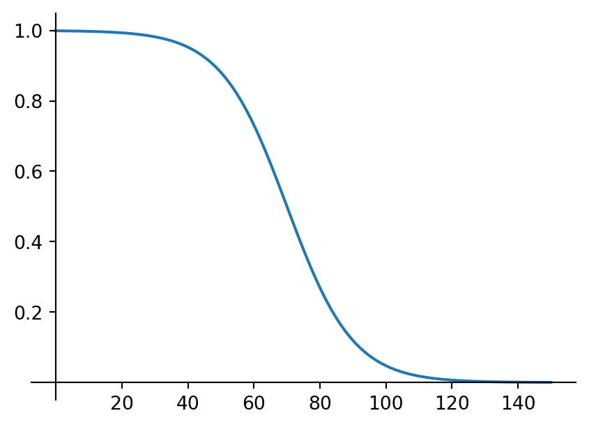
If we were building (for convenience) a one-factor (cf. Definition 10.1 v), exchangeable Bernoulli mixture model with the CCI as only common factor represented by the random variable \(\Psi\) then we’d hence set \(\Psi \sim \mathcal{N}(102,5)\). For the individual default probability function \(\pi\) (applying to all \(m\) obligors i.e. companies in the retail sector, as the model is exchangeable) you’d want a choice that reflects the logic that the larger the CCI during the coming year/the value \(\psi\) that \(\Psi\) takes, the smaller the default probability \(\pi(\psi)\). So it should be a decreasing function. A possible choice could be \[\pi(\psi)=\frac{1}{1+e^{0.1(\psi-70)}} \quad \text{for all } \psi \in \R,\] see Figure 10.1. If we would assume that the CCI remains stable over the coming year at level 102 i.e. we’d condition on \(\Psi=102\), then the default probability for each of the \(m\) obligors is \[\pi(102) \approx 0.039\] and we see confirmed in the plot that this default probability would be higher resp. lower if \(\Psi\) would take a value smaller than resp. larger than 102.
Let’s list some famous ones with fancy names!
Example 10.2 There are some prominent specific combinations of distributions for \(\Psi\) and individual default probability functions \(\pi\) in one-factor exchangeable Bernoulli mixture models that are worth pointing out:
- Beta mixture model: \(\Psi\) follows a Beta distribution and \(\pi(\psi)=\psi\);
- Probit-normal mixture model: \(\Psi \sim \mathcal{N}(0,1)\) and \(\pi(\psi)=\Phi(a+b\psi)\), where \(\Phi\) is the cdf of a standard Normal distribution and \(a,b \in \R\) are parameters;
- Logit-normal mixture model: \(\Psi \sim \mathcal{N}(0,1)\) and \[\pi(\psi)=\frac{1}{1+e^{a+b\psi}},\] where \(a,b \in \R\) are parameters.
Note that in such models, there is some freedom in how the internals, i.e. \(\Psi\) and \(\pi\), are exactly scaled/normalised. What ultimately matters is the random variable \(\pi(\Psi)\): any two models for which this is the same random variable are equivalent in the sense that the default indicators (cf. Definition 10.1 i) have the same distributions in either model (and that’s all that matters for drawing conclusions from the model).
So for instance, if model 1 uses a \(\Psi\) and a \(\pi\), and model 2 uses \(\widehat{\Psi}:=a\Psi+b\) and \(\widehat{\pi}(\psi):=\pi((\psi-b)/a)\), then these are equivalent models because \[\widehat{\pi}(\widehat{\Psi})=\pi \left( \frac{\widehat{\Psi}-b}{a} \right)=\pi \left( \frac{a\Psi+b-b}{a} \right)=\pi(\Psi).\]
The model in Example 10.1 is a nice example of this: it is equivalent to a logit-normal mixture model as introduced above.
Example 10.3 The global investment bank Credit Suisse, nowadays part of another investment bank called UBS, has a famous credit risk model called CreditRisk+. It is a Bernoulli mixture model, in which the common factors \(\Psi_1, \ldots, \Psi_p\) are independent random variables with Gamma distributions, and the individual default probability functions are of the form \[\pi_i(\psi_1,\ldots,\psi_p) = 1-e^{-(w^{(i)}_1 \psi_1+\ldots+w^{(i)}_p \psi_p)},\] where \(w^{(i)}_1, \ldots, w^{(i)}_p>0\) are parameters specific for the \(i\)-th obligor.
Much like Moody’s KMV model (cf. Section 9.4), this model is not so much very sophisticated or complicated, what makes it particularly powerful in Credit Suisse’s hands is their large collections of (proprietary) data to calibrate their model against and their experience in working with it.
10.4 Computations in Bernoulli mixture models
Now we have firmly introduced Bernoulli mixture models in the above two sections, it is time to do some nice analysis! What our risk manager is ultimately interested in is the probability that a particular obligor defaults, or that multiple obligors default simultanuously, or how many of the olbligors will default etc. In this section we’ll work through a number of examples to see how to work out the answers to such questions.
Remark 10.1. As we embark on exploring such questions, it is good to be fully aware of the folllowing. A Bernoulli mixture model (cf. Definition 10.2) models whether or not each obligor survives the coming year as a probabilistic experiment which we can consider unfolding in several steps as follows:
- Each of the common factors (random variables) \(\Psi_1, ..., \Psi_p\) takes a value, say \(\psi_1, \ldots, \psi_p\) (real numbers).
- The values \(\pi_1(\psi_1, \ldots, \psi_p)\), …, \(\pi_m(\psi_1, \ldots, \psi_p)\) are computed (each a real number from the interval \([0,1]\)).
- The values computed in step 2 feed as parameters into the Bernoulli distributions that the default indicators \(Y_1, \ldots, Y_m\) have (cf. Equation 10.2) and hence we now fully know their distribution. Each \(Y_1, \ldots, Y_m\) takes a value (either \(0\) or \(1\)) and hence we know which (if any) of the \(m\) obligors have ended up defaulting.
In general, if we have a random variable from which we produce a sample/realisation and then plug it into some function, we could (of course) equally well apply that function to our random variable to produce a new random variable and just generate a sample/realisation from that new random variable. Same difference eh!
So, equivalently, steps 1 & 2 above could be combined into a single step to get the following stepwise execution:
- Each of the random variables \(\pi_1(\Psi_1, \ldots, \Psi_p)\), \(\pi_2(\Psi_1, \ldots, \Psi_p)\), …, \(\pi_m(\Psi_1, \ldots, \Psi_p)\) takes a value (each a real number from the interval \([0,1]\)).
- The values computed in step i feed as parameters into the Bernoulli distributions that the default indicators \(Y_1, \ldots, Y_m\) have (cf. Equation 10.2) and hence we now fully know their distribution. Each \(Y_1, \ldots, Y_m\) takes a value (either \(0\) or \(1\)) and hence we know which (if any) of the \(m\) obligors have ended up defaulting.
The key point is: one “run” of this probabilistic experiment requires a chain of twice generating a set of samples/realisations, where the second phase (the \(Y_i\)’s) depends on what happened in the first phase. This means that we can’t just focus on the \(Y_i\)’s in isolation: their distribution depends on what happens in the first phase after all!
So how do we compute say the probability that the first obliger defaults i.e. \(\P(Y_1=1)\)? The intuitively appealing strategy is: for any possible set of samples/realisations \(\psi_1,\ldots,\psi_p\) of \(\Psi_1,\ldots,\Psi_p\), determine the probability that the first obligor defaults given that we get to see this set of samples/realisations in phase 1 i.e. \[\P(Y_1=1 \, | \, \Psi_1=\psi_1, \ \Psi_2=\psi_2, \ldots, \Psi_p=\psi_p) \tag{10.4}\] (which is straightforward, recall from Definition 10.2) and then “average out” the probabilities Equation 10.4 over all possible sets of samples/realisations from \(\Psi_1,\ldots,\Psi_p\) to get your hands on \(\P(Y_1=1)\). Mathematically we already know exactly how to carry out this strategy: it is (of course!) nothing but the Law of Total Expectation (cf. Section A.4.2) — this guy will be your main friend in the below so keep him close!
10.4.1 Computations with the default indicators
Example 10.4 In this example we look at a version of the CreditRisk+ model we mentioned in Example 10.3: an exchangeable Bernoulli mixture model with two factors \(\Psi_1\) and \(\Psi_2\), independent and both \(\text{Exp}(1)\) distributed, and with individual default probability function \(\pi\) given by \[\pi(\psi_1,\psi_2)=1-e^{-(c_1 \psi_1 + c_2 \psi_2)} \quad \text{for all } \psi_1, \psi_2>0 \tag{10.5}\] (since \(\Psi_1\) and \(\Psi_2\) have range \((0,\infty)\), we only need to define \(\pi\) for positive argument values), where \(c_1, c_2 \geq 0\) are parameters.
The probability that an obligor defaults. Let’s first look at the probability that obligor \(i\) defaults i.e. \(\P(Y_i=1)\). Recall the strategy outlined in Remark 10.1: using the Law of Total Expectation (cf. Section A.4.2) we write (cf. Equation A.50 & Equation A.51, and also Remark A.3) \[\P(Y_i=1)=\E[\varphi(\Psi_1,\Psi_2)], \tag{10.6}\] where \(\varphi\) is the function defined as \[\varphi(\psi_1,\psi_2)=\P(Y_i=1 \, | \, \Psi_1=\psi_1, \ \Psi_2=\psi_2) \quad \text{for all } \psi_1, \psi_2>0.\] We can work out this definition as follows, recalling Equation 10.3 and using the fact that the model is exchangeable, for any \(\psi_1, \psi_2>0\): \[\varphi(\psi_1,\psi_2)=\pi_i(\psi_1,\psi_2)=\pi(\psi_1,\psi_2)=1-e^{-(c_1 \psi_1 + c_2 \psi_2)}.\] Plugging this back into Equation 10.6 we hence get \[\P(Y_i=1)=\E \left[ 1-e^{-(c_1 \Psi_1 + c_2 \Psi_2)} \right] \tag{10.7}\] and it remains to work out this bastard.
For any expectation involving two or more random variables, we have two standard tools: working out the appropriate higher dimensional integral (cf. Equation A.40), or using the Law of Total Probability again (conditioning on one of the two random variables taking a certain value). Let’s go down the integral route (but the other route is equally viable if you’d prefer). Observe that since \(\Psi_1\) and \(\Psi_2\) are independent and both \(\text{Exp}(1)\) distributed, their joint pdf \(f_{\Psi_1,\Psi_2}\) is the product of the individual \(\text{Exp}(1)\) pdf’s (recall Section A.5, and Appendix B if needed): \[\begin{align*} f_{\Psi_1,\Psi_2}(\psi_1,\psi_2) &= f_{\Psi_1}(\psi_1) f_{\Psi_2}(\psi_2) \\ &= \begin{cases} e^{-\psi_1} & \text{if } \psi_1>0 \\ 0 & \text{if } \psi_1 \leq 0 \end{cases} \cdot \begin{cases} e^{-\psi_2} & \text{if } \psi_2>0 \\ 0 & \text{if } \psi_2 \leq 0 \end{cases} \\ &= \begin{cases} e^{-\psi_1-\psi_2} & \text{if } \psi_1>0 \text{ and } \psi_2>0 \\ 0 & \text{otherwise}. \end{cases} \end{align*} \tag{10.8}\] So, applying Equation A.40 to Equation 10.7 we can compute (recall the brief discussion of double integrals in Section A.3.2 if you’d like a refresher) \[\begin{align*} \P(Y_i=1) &= \E \left[ 1-e^{-(c_1 \Psi_1 + c_2 \Psi_2)} \right] \\ &= \iint_{\R^2} \left( 1-e^{-(c_1 \psi_1 + c_2 \psi_2)} \right) f_{\Psi_1,\Psi_2}(\psi_1,\psi_2) \d (\psi_1,\psi_2) \\ &= \int_0^\infty \int_0^\infty \left( 1-e^{-(c_1 \psi_1 + c_2 \psi_2)} \right) e^{-\psi_1-\psi_2} \d \psi_1 \d \psi_2 \\ &= \int_0^\infty \int_0^\infty \left( e^{-\psi_1-\psi_2}-e^{-(c_1+1) \psi_1 - (c_2+1) \psi_2} \right) \d \psi_1 \d \psi_2 \\ &= \int_0^\infty \left[ -e^{-\psi_1-\psi_2} + \frac{1}{c_1+1} e^{-(c_1+1) \psi_1 - (c_2+1) \psi_2)} \right]_{\psi_1=0}^{\psi_1=\infty} \d \psi_2 \\ &= \int_0^\infty e^{-\psi_2} - \frac{1}{c_1+1} e^{- (c_2+1) \psi_2} \d \psi_2 \\ &= \left. -e^{-\psi_2} + \frac{1}{(c_1+1)(c_2+1)} e^{- (c_2+1) \psi_2} \right|_{\psi_2=0}^{\psi_2=\infty} \\ &= 1-\frac{1}{(c_1+1)(c_2+1)}. \end{align*} \tag{10.9}\]
Breath in, breath out — there we finally are! A bit of a sanity check is always good of course — in this case, as we’ve been computing a probability the result should be an element from \([0,1]\). Indeed it is readily clear that the final expression is above is bounded above by \(1\), and its smallest value is achieved for \(c_1=c_2=0\) in which case the above expression simplifies to \(0\). It’s also worthwhile to note that while we set out to compute the probability that the \(i\)-th obligor defaults, i.e. \(\P(Y_i=1)\), the final expression does not depend on \(i\). That is explained by the fact that we’re looking at an exchangeable model, in which case each obligor has the same individual default probability function and hence the same probability of default.
The probability that multiple obligors default. Feeling a bit more confident after hammering out the above nice computation, let’s pick out two obligers, say \(i\) and \(j\), and let’s wonder what the probability is that these both default (the principle used here applies in the same way to more than two) i.e. what \(\P(Y_i=1 \ \& \ Y_j=1)\) is.
For the same reasons as above and as explained in Remark 10.1, we’ll again need to go down the Law of Total Expectation route (i.e. Equation A.50 & Equation A.51, and also Remark A.3): we have that \[\P(Y_i=1 \ \& \ Y_j=1)=\E[\varphi(\Psi_1,\Psi_2)], \tag{10.10}\] where the function \(\varphi\) is defined as \[\varphi(\psi_1,\psi_2)=\P(Y_i=1 \ \& \ Y_j=1 \, | \, \Psi_1=\psi_1, \ \Psi_2=\psi_2) \quad \text{for all } \psi_1, \psi_2>0.\] To work out \(\varphi\), we can use that with the conditioning in place (!), \(Y_i\) and \(Y_j\) are independent (cf. Definition 10.1 iv) so that \[\begin{align*} \varphi(\psi_1,\psi_2) &= \P(Y_i=1 \ \& \ Y_j=1 \, | \, \Psi_1=\psi_1, \ \Psi_2=\psi_2) \\ &= \P(Y_i=1 \, | \, \Psi_1=\psi_1, \ \Psi_2=\psi_2) \P(Y_j=1 \, | \, \Psi_1=\psi_1, \ \Psi_2=\psi_2) \\ &= \pi_i(\psi_1,\psi_2) \pi_j(\psi_1,\psi_2) \\ &= \pi(\psi_1,\psi_2)^2 \\ &= \left( 1-e^{-(c_1 \psi_1 + c_2 \psi_2)} \right)^2, \end{align*} \] where the second equality uses the conditional independence mentioned above, the third Equation 10.3 again, the fourth that the model is exchangeable and the fifth the given expression for \(\pi\).
So now we can (again) work out Equation 10.10 as a double integral (relying on Equation A.40), where the joint pdf \(f_{\Psi_1,\Psi_2}\) is of course unchanged from above: \[\begin{align*} \P(Y_i=1 \ \& \ Y_j=1) &= \E \left[ \left( 1-e^{-(c_1 \Psi_1 + c_2 \Psi_2)} \right)^2 \right] \\ &= \iint_{\R^2} \left( 1-e^{-(c_1 \psi_1 + c_2 \psi_2)} \right)^2 f_{\Psi_1,\Psi_2}(\psi_1,\psi_2) \d (\psi_1,\psi_2) \\ &= 1-\frac{2}{(c_1+1)(c_2+1)}+\frac{1}{(2 c_1+1)(2 c_2+1)}. \end{align*} \tag{10.11}\] For the working of the integral in Equation 10.11, after working out the brackets, you could either just go full steam ahead with the algebra or you could be slightly smart. First note that \[\iint_{\R^2} f_{\Psi_1,\Psi_2}(\psi_1,\psi_2) \d (\psi_1,\psi_2)=1\] (any (joint) pdf integrates to \(1\) after all). Further \[\begin{align*} 1 &- \iint_{\R^2} e^{-(c_1 \psi_1 + c_2 \psi_2)} f_{\Psi_1,\Psi_2}(\psi_1,\psi_2) \d (\psi_1,\psi_2) \\ &\qquad = \iint_{\R^2} f_{\Psi_1,\Psi_2}(\psi_1,\psi_2) \d (\psi_1,\psi_2) \\ &\qquad \qquad - \iint_{\R^2} e^{-(c_1 \psi_1 + c_2 \psi_2)} f_{\Psi_1,\Psi_2}(\psi_1,\psi_2) \d (\psi_1,\psi_2) \\ &\qquad = \iint_{\R^2} \left( 1-e^{-(c_1 \psi_1 + c_2 \psi_2)} \right) f_{\Psi_1,\Psi_2}(\psi_1,\psi_2) \d (\psi_1,\psi_2) \\ &\qquad = 1-\frac{1}{(c_1+1)(c_2+1)} \end{align*} \] (the final equality borrowed from the above integral computation) so that \[\iint_{\R^2} e^{-(c_1 \psi_1 + c_2 \psi_2)} f_{\Psi_1,\Psi_2}(\psi_1,\psi_2) \d (\psi_1,\psi_2) = \frac{1}{(c_1+1)(c_2+1)} \tag{10.12}\] and then hence also \[\iint_{\R^2} e^{-(2 c_1 \psi_1 + 2 c_2 \psi_2)} f_{\Psi_1,\Psi_2}(\psi_1,\psi_2) \d (\psi_1,\psi_2) = \frac{1}{(2 c_1+1)(2 c_2+1)}.\]
In whatever way you decide to work it out, Equation 10.11 gives us a fascinating expression for the probability that both obligors \(i\) and \(j\) default! Or, in fact, since the model is exchangeable, the probability that any two obligors you select will both default.
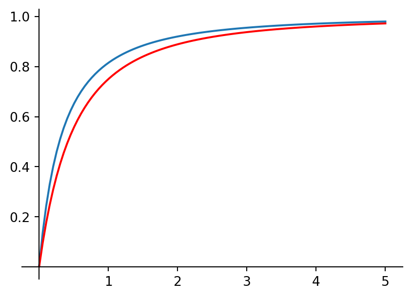
And note that \[\begin{align*} \P(Y_i=1 \ \& \ Y_j=1) &= 1-\frac{2}{(c_1+1)(c_2+1)}+\frac{1}{(2 c_1+1)(2 c_2+1)} \\ &\not= \left( 1-\frac{1}{(c_1+1)(c_2+1)} \right)^2 = \P(Y_i=1) \P(Y_j=1), \end{align*} \] confirming that without any conditioning, \(Y_i\) and \(Y_j\) are not independent as already mentioned in the second “note” in Definition 10.1! In fact, with a little bit of algebra and/or a plot you can check that for any \(c_1, c_2 >0\) it holds that \[\P(Y_i=1 \ \& \ Y_j=1)>\P(Y_i=1) \P(Y_j=1)\] or equivalently that (just by def of the conditional expectation Equation A.42 and that \(\P(Y_i=1)=\P(Y_j=1)\)) \[\P(Y_j=1 \, | \, Y_i=1)>\P(Y_j=1)\] (see also Figure 10.2). This is because of a “feedback loop” if you will: given that the \(i\)-th obligor defaults, it is more likely that the common factors are having “bad news” values, which in turn makes it more likely that obligor \(j\) defaults than it would have been without that bit of knowledge about the \(i\)-th obligor/the common factor values. (Indeed, the presence of the common factors in this model cause \(Y_i\) and \(Y_j\) to have a positive value for Kendall’s tau i.e. to exhibit more concordant than discordant behaviour in terminology of Section 5.3! :)).
10.4.2 Computations with the number of defaulting obligors
Recall from Definition 10.1 that in a mixture model with \(m\) obligors, the number of obligors that default is given by the expression \[N=\sum_{i=1}^m Y_i.\] As already mentioned in the “notes” in Definition 10.1, even though the \(Y_i\)’s are always \(\{0,1\}\)-valued random variables, the other conditions for \(N\) to have a Binomial distribution are not necessarily satisfied.
However in the special case of an exchangeable Bernoulli mixture model, at least given/conditional on \(\Psi_1=\psi_1\), …, \(\Psi_p=\psi_p\) we have that the \(Y_i\)’s are i.i.d., each with “success” (=default) probability \(\pi(\psi_1,\ldots,\psi_p)\) (cf. Definition 10.2) and hence then \(N\) does have a Binomial distribution, with pameters \(m\) (the number of obligors/experiments) and \(\pi(\psi_1,\ldots,\psi_p)\) (the “success”/default probability per experiment). So:
Proposition 10.1 In an exchangeable Bernoulli mixture model from Definition 10.2, the (random) number of defaults among the \(m\) obligors expressed as \[N=\sum_{i=1}^m Y_i\] has the property that given/conditional on \(\Psi_1=\psi_1\), …, \(\Psi_p=\psi_p\), \[N \sim \text{Binomial}(m,\pi(\psi_1,\ldots,\psi_p)).\]
In this setting we can work out probs/expectations for \(N\), using the same strategy as we also used in Section 10.4.1: first condition on \(\Psi_1=\psi_1\), …, \(\Psi_p=\psi_p\) (for any \(\psi_1,\ldots,\psi_p\)), compute the prob/expectation you’re interested in using the Binomial distribution from Proposition 10.1, and then use the Law of Total Expectation to “average out” over all \(\psi_1,\ldots,\psi_p\) to get the original prob/expectation for \(N\) you’re interested in. For example:
Example 10.5 Consider again the exchangeable Bernoulli mixture model from Example 10.4, and let’s look at the (random) number of obligors that defaults: \[N=\sum_{i=1}^m Y_i.\]
The probability that exactly one obligor defaults. Let’s compute \(\P(N=1)\). Appealing to our unsung hero the Law of Total Expectation, cf. Equation A.50 & Equation A.51, we can write \[\P(N=1)=\E[\varphi(\Psi_1,\Psi_2)] \tag{10.13}\] where the function \(\varphi\) is defined as \[\varphi(\psi_1,\psi_2)=\P(N=1 \, | \, \Psi_1=\psi_1, \ \Psi_2=\psi_2) \quad \text{for all } \psi_1, \psi_2>0.\]
Working out \(\varphi\), using Proposition 10.1 (and the pmf from Appendix B if needs be), for any \(\psi_1, \psi_2>0\): \[\begin{align*} \varphi(\psi_1,\psi_2) &= \P(N=1 \, | \, \Psi_1=\psi_1, \ \Psi_2=\psi_2) \\ &= \binom{m}{1} \pi(\psi_1,\psi_2) \big( 1-\pi(\psi_1,\psi_2) \big)^{m-1} \\ &= m \left( 1-e^{-(c_1 \psi_1 + c_2 \psi_2)} \right) e^{-(m-1)(c_1 \psi_1 + c_2 \psi_2)} \\ &= m \left( e^{-(m-1)(c_1 \psi_1 + c_2 \psi_2)} - e^{-m(c_1 \psi_1 + c_2 \psi_2)} \right), \end{align*} \] where we also used the expression for the individual default probability function \(\pi\) from Equation 10.5.
Now going back to Equation 10.13, appealing to Equation A.40 we write it as a double integral also involving the joint pdf \(f_{\Psi_1,\Psi_2}\) of \(\Psi_1\) and \(\Psi_2\): \[\begin{align*} \P(N=1) &= \E[\varphi(\Psi_1,\Psi_2)] \\ &= \iint_{\R^2} \varphi(\psi_1,\psi_2) f_{\Psi_1,\Psi_2}(\psi_1,\psi_2) \d (\psi_1,\psi_2) \end{align*} \] and then it is again “just” a matter of plugging in the above expression for \(\varphi\) and \(f_{\Psi_1,\Psi_2}\) (recall we already found an expression for this guy in Equation 10.8) working out this bastard to get to our final expression. Of course we can always get the elbow grease out and hammer our way through, but since we can write the integral as \[\begin{align*} \P(N=1) &= m \int_0^\infty \int_0^\infty e^{-(c_1(m-1) \psi_1 + c_2(m-1) \psi_2)} f_{\Psi_1,\Psi_2}(\psi_1,\psi_2) \d \psi_1 \d \psi_2 \\ & \qquad - m \int_0^\infty \int_0^\infty e^{-(c_1 m \psi_1 + c_2 m \psi_2)} f_{\Psi_1,\Psi_2}(\psi_1,\psi_2) \d \psi_1 \d \psi_2 \end{align*} \] we can also turn to Equation 10.12 to immediately work this out to \[\begin{align*} \P(N=1) &= \frac{m}{\big( c_1(m-1)+1 \big) \big( c_2(m-1)+1 \big)} \\ &\qquad -\frac{m}{( c_1 m+1 ) ( c_2 m+1 )}. \end{align*} \]
Not very pretty, but eh, who are we to judge! As a bit of a sanity check, note that if we sub in \(m=1\) then \(\P(N=1)\) simplifies to \(1-1/((c_1+1)(c_2+1))\) and that is identical to the probability that any of the obligor defaults, as computed in Example 10.4. And that makes perfect sense of course: if \(m=1\) i.e. there is only one obligor in total, then the event that exactly one obligor defaults is the same thing as that one obligor defaulting.
The expected number of obligors that default. We can also do \(\E[N]\) — again via the Law of Total Probability (now Equation A.48 & Equation A.49): \[\E[N]=\E[\varphi(\Psi_1,\Psi_2)] \tag{10.14}\] where the function \(\varphi\) is defined as \[\varphi(\psi_1,\psi_2)=\E[N \, | \, \Psi_1=\psi_1, \ \Psi_2=\psi_2] \quad \text{for all } \psi_1, \psi_2>0.\] From Proposition 10.1 we know that in \(\varphi\), we’re taking the expectation of a \(\text{Binomial}(m,\pi(\psi_1,\psi_2))\) which is just the product of the parameters (recall from Appendix B if needs be) i.e. for any \(\psi_1, \psi_2>0\): \[\varphi(\psi_1,\psi_2)=m \pi(\psi_1,\psi_2) = m \left( 1-e^{-(c_1 \psi_1+c_2 \psi_2)} \right)\] (recall \(\pi\) from Equation 10.5). Plugging this back into Equation 10.14 yields \[\E[N]=m \E \left[ 1-e^{-(c_1 \Psi_1+c_2 \Psi_2)} \right].\] So yet another double integral?? Well yes, sorry :( — but we’ve done this one already in Equation 10.9 so we can just copy from there: \[\E[N]=m \left( 1-\frac{1}{(c_1+1)(c_2+1)} \right). \tag{10.15}\]
Obviously with these techniques we can in principle attack any probability and also any expectation of (a function of) \(N\)! :).
10.5 The risk manager’s perspective
In the above sections we’ve done a deep dive into Bernoulli mixture models, in particular focussing on exchangeable ones. They form a powerful and rich collection of models, but if we come back to the surface and go sit in the risk manager’s chair again there is still a piece of the puzzle missing. Namely, our beautiful Bernoulli mixture model only looks at which obligors are going to default. And as risk manager that’s not the only thing we want to know, we are above all interested in the bottom line: how much the defaults (if any) among our obligors is going to cost us! So let’s add that to our model.
For the main focus in this section, we make an assumption on the group of \(m\) obligors to make our lives not too complicated:
Definition 10.3 We say that a group of obligors have identical characteristics (note: non-standard terminology to the best of my knowledge) if:
- their default probabilities can be modelled using an exchangeable Bernoulli mixture model as defined in Definition 10.2, and
- the financial obligation to which these default probabilities apply are identical (for example, each obligor has to repay a loan of the same amount).
Now suppose that our \(m\) obligors have identical characteristics as laid out in Definition 10.3. Then they are essentially interchangeable parties for us: we only care about how many of them default, not which ones exactly. Let \(L\) be a non-negative random variable which models the amount of money we stand to lose due to an obligor defaulting. It makes sense for this to be random in general, because as discussed in Section 9.1, default does not necessarily mean that we get no money at all but rather less than what was actually agreed. So \(L\) models the difference between the outstanding obligation and how much we actually end up receiving i.e. in terms of the terminology in Section 9.1: \[L=\text{LGD} \cdot \text{EAD}.\]
Let’s link this up with an exchangeable Bernoulli mixture model as defined in Definition 10.2. Then for each of the \(m\) obligors that defaults, our loss is modelled by \(L\). As the loss suffered due to one defaulting obligor does not influence the loss suffered due to another defaulting obligor, each default of an obligor adds an independent copy of \(L\) to our total loss. Recall from Definition 10.1 ii that we use \(N\) to denote the (random) number of obligors that will default, and hence our total loss due to defaults i.e. our (total) credit risk \(X\) for this group of \(m\) obligors is given by \[X=\sum_{k=1}^N L_k, \tag{10.16}\] where \(L_1, L_2, \ldots\) are independent copies of \(L\) (and also independent of our Bernoulli mixture model) and we naturally understand \(X=0\) if \(N=0\) in Equation 10.17.
So here it is: this \(X\) is the cherry on top of our credit risk cake, our centerpiece, the rug that really ties the room together!1 But yeah, Equation 10.17 does look like a bit of a complicated expression: a sum of i.i.d. random variables but containing a random (namely, \(N\)) number of terms… Oh but hang on, that actually rings a bell! Well indeed, \(X\) as defined in Equation 10.17 has nothing but a compound distribution as we encountered before, in Section 7.3! And though that was not necessarily in the same context, the maths doesn’t care in the slightest about context: every result about compound distributions that we have proven with our own blood, sweat and tears in Section 7.3 is equally valid in this context — in particular, Proposition 7.2 lists the fundamental techniques available for computing probabilities and expectations for \(X\), and Theorem 7.1 provides ready to take away formulas for the moment generating function, mean and variance of \(X\)! Don’t you just love it when a plan comes together?2
1 What, you haven’t seen the movie “The Big Lebowski”? Come on!
2 “The A-Team” people!
Proposition 10.2 Consider a group of \(m\) obligors with identical characteristics (cf. Definition 10.3), and a model consisting of the following two parts.
- An exchangeable Bernoulli mixture model (cf. Definition 10.2) describing which (if any) obligors will default, with \(N\) (cf. Definition 10.1 ii) denoting the number of obligors that will default.
- A non-negative random variable \(L\), independent of the Bernoulli mixture model, describing the loss suffered due to an obligor defaulting (i.e. \(L=\text{LGD} \cdot \text{EAD}\), cf. Section 9.1).
Then the (total) credit risk \(X\) resulting from this group of obligors can be expressed as \[X=\sum_{k=1}^N L_k, \tag{10.17}\] where \(L_1, L_2, \ldots\) are independent copies of \(L\) (i.e. they are i.i.d.) and we naturally understand \(X=0\) if \(N=0\).
Note that this \(X\) has a compound distribution as defined in Definition 7.1, and hence both Proposition 7.2 and Theorem 7.1 are available for analysing \(X\).
If our obligors do not have identical characteristics then an expression for \(X\) is discussed in Remark 10.2.
Here’s a quick example:
Example 10.6 Consider a group of \(m\) obligors who have all taken out a loan with you, for say \(£K\) (a constant). This \(£K\) is hence also your Exposure At Default (EAD), cf. Section 9.1. You model the Loss Given Default (LGD), i.e. the fraction of the loan you won’t get back in case of default (cf. Section 9.1), by a \(\text{Unif}(0,1)\) distribution.
Further suppose that the default probabilities can be modelled using the exchangeable Bernoulli mixture model we already studied in Example 10.4 and Example 10.5.
You denote by \(X\) your credit risk for this group of obligors.
Now, note that the conditions in Definition 10.3 are satisfied, i.e. these obligors have identical characteristics. Hence we get from Proposition 10.2 that we can write \(X\) as the compound distribution \[X=\sum_{k=1}^N L_k, \tag{10.18}\] where \(N\) is the (random) number of defaults and \(L_1, L_2, \ldots\) are independent copies of the loss-upon-default random variable \(L\) given by \[L=\text{LGD} \cdot \text{EAD}=U \cdot K,\] where \(U \sim \text{Unif}(0,1)\).
The probability of no credit risk loss. You suffer no loss at all if it holds true that \(X=0\) i.e. if (and only if) \(N=0\) — because, if \(N=0\) then \(X=0\) by convention (cf. Proposition 10.2) while if \(N \geq 1\) i.e. at least one obligor defaults then you will definitely lose some positive amount, this is clear from the story context but also from Equation 10.18. So, we’re after the probability \[\P(X=0)=\P(N=0).\] Now recall that \(N\) comes from the Bernoulli mixture model, and analysing it generally requires some work: conditioning on the common factors and yada yada, we saw some examples of that in Example 10.5. Going down that road one more time, following exactly the same strategy as in Example 10.5 (so you can fill in any missing details yourself!): we have that \[\P(N=0)=\E[\varphi(\Psi_1,\Psi_2)],\] where \[\begin{align*} \varphi(\psi_1,\psi_2) &= \P(N=0 \, | \, \Psi_1=\psi_1, \ \Psi_2=\psi_2) \\ &= \left( 1-\pi(\psi_1,\psi_2) \right)^m \\ &= e^{-m(c_1 \psi_1 + c_2 \psi_2)} \end{align*} \] and hence \[\P(N=0)=\E \left[ e^{-m(c_1 \Psi_1 + c_2 \Psi_2)} \right]=\frac{1}{(c_1 m+1)(c_2 m+1)}.\] So in conclusion: the probability that you will suffer no loss at all is \[\P(X=0)=\frac{1}{(c_1 m+1)(c_2 m+1)}.\] Note how this probability decreases pretty rapidly as \(m\) increases, giving you the obvious message that the more people you lend that \(£K\) to, the more likely it is you will lose at least some of it due to default(s)!
The expected loss due to credit risk. We could also look at computing \(\E[X]\)! Here Proposition 10.2 comes in particularly handy: it tells us that for the compound distribution Equation 10.18, we shouldn’t forget that we have both Proposition 7.2 and Theorem 7.1 available. Indeed Theorem 7.1 gives us a ready to pick up expression for \(\E[X]\), namely (cf. Equation 7.27) \[\E[X]=\E[N] \E[L_1].\] Recall that \(L_1\) is a copy of \(L\) and hence \[\E[L_1]=\E[L]=\E[U \cdot K]=\E[U] \cdot K=\frac{K}{2}\] (recall the expectation of a Uniform distribution from Appendix B if needs be). Furthermore, we had already computed \(\E[N]\) in Example 10.5, cf. Equation 10.15. So this one is nice and quick and gives us that \[\E[X]=\frac{mK}{2} \left( 1-\frac{1}{(c_1 +1)(c_2 +1)} \right).\]
Finally then, a brief discussion of how to deal with the total credit risk if we drop the assumption that our obligors have identical characteristics:
Remark 10.2. Our assumption that Definition 10.3 applies makes the resulting expression for the credit risk very elegant and accessible for analysis with available tools. If we were to drop this assumption and consider any group of \(m\) obligors rather, then this results in (at least one of) two changes:
- In the Bernoulli mixture model, it may no longer be feasible to assume that they share the same individual default probability function in which case our model is no longer exchangeable.
- It may no longer be accurate enough to use the same distribution for the loss each obligor causes upon default i.e. we may need to assign each obligor their own loss-upon-default random variable, say \(L_1, \ldots, L_m\). These will normally still be independent, but would no longer necessarily have the same distribution — for instance, in case different obligors have different outstanding obligations to you as risk manager.
We could in this case still write down a compact expression for the total credit risk \(X\), namely \[X=\sum_{i=1}^m Y_i L_i, \tag{10.19}\] where the \(Y_i\)’s are the default indicators (cf. Definition 10.1 i). Note the logic of this expression: the counter \(i\) walks through our list of obligors, if the \(i\)-th obligor defaults (i.e. \(Y_i=1\) so that \(Y_i L_i=L_i\)) then the corresponding loss \(L_i\) is added to \(X\) while if they don’t default (i.e. \(Y_i=0\) so that \(Y_i L_i=0\)) nothing gets added to \(X\).
The problem with Equation 10.19 is that the \(Y_i\)’s are generally not independent (recall from the “notes” in Definition 10.1) and now the \(L_i\)’s are not necessarily identically distributed. So \(X\) could very well be a sum of random variables that are neither independent nor identically distributed! That doesn’t necessarily mean that we can’t analyse such an expression at all, it’s just that we’d typically have to work from “first principles” and it can easily get a lot more messy & hard work than our elegant compound distribution in Proposition 10.2!
10.6 Some exercises
NoteAbout the exercises
Each exercise has a (rough) indication of its difficulty, as follows:
| * | easier: can be solved by (almost) only using relevant definitions/results, |
| ** | medium: in addition to relevant definitions/results, needs a limited amount of work/creativity, |
| *** | harder: in addition to relevant definitions/results, needs a larger amount of work/serious creativity, |
| 💀 | warning: might make your brain hurt! These are mainly intended to provide some extra challenge for those of you keen on that and are generally quite hard. You don't need to worry about these too much for exam purposes. |
The exam consists of mostly ** and *** level questions, some *, and possibly at most a few marks worth of 💀.
A bit of preaching: it is an incredibly important part of the study process to try and work on the exercises as much as possible. To become a better mathematician/learn new maths (and also to get a good exam mark ;)), above all you need to do it. And yes, of course that includes falling over things, and making mistakes, and getting stuck, and getting frustrated — all part of the game and what you’re supposed to be doing! Your lecturers have done that as well and still do it. What matters is that you don’t let that discourage you and that you make good use of the help and resources available to help you develop your skills. As part of that, many exercises have a hint in a block like this:
NoteHint (click to view)
Hint!
These are trying to help you on your way if you don’t know where to start or to provide some ideas if you get stuck. In spirit of the above, always have a look at these first and try again before you look at the full solution. (These hints are an extra service that won’t be available in the exam I’m afraid ;).)
Of course, we have our classes and there’s office hours, email etc. as well — I’m at any time very happy to help you with any questions you may have, and you should please never feel that any question is “too dumb” to ask!
Full/detailed solutions for the exercises will become available, just immediately below the exercises, immediately after our tutorial hour (you may have to refresh the page).
Exercise 10.1 [**/***] Consider one more time the exchangeable Bernoulli mixture model for \(m\) obligors based on the CreditRisk+ model we already discussed in Example 10.3, Example 10.4, Example 10.5 and Example 10.6. If you don’t have these examples very sharp for yourself anymore, then have a reread of them first!
- Fix some \(i \in \{1,\ldots,m\}\). Compute the probability that the \(i\)-th obligor does not default.
- Now consider two obligors \(i, j \in \{1,\ldots,m\}\). We are interested in the (joint) probability that the \(i\)-th obligor defaults and the \(j\)-th obligor does not default. Why can we not compute this as the product of the probability that the \(i\)-th obligor defaults with the probability that the \(j\)-th obligor does not default? Compute the probability that we are interested in.
- Suppose that each of the \(m\) obligors has the obligation to pay you back a loan of £1,000, and assume that the loss given default is 100%. What is the expectation of your credit risk?
NoteHint (click to view)
Before starting this question, make sure to remind yourself of the ingredients of this model, cf. Example 10.3 and you also want to review the techniques/ideas used in the other examples mentioned in the question!
For part i, note that we’re asked to compute \(\P(Y_i=0)\). There’s a quick and not so quick way ;). Maybe you want to explore both! For the quick way, observe that we have already computed \(\P(Y_i=1)\) (cf. Equation 10.9) so that, if you recall Definition 10.1 if needs be, you can immediately write down \(\P(Y_i=0)\) as well. For the not so quick way, we simply need to work out this prob from scratch. For this, just follow exactly the same ideas as we used to get to Equation 10.9 in Example 10.4.
For part ii, now we’re asked to compute \(\P(Y_i=1 \ \& \ Y_j=0)\). For the first question, that would be perfectly viable if \(Y_i\) and \(Y_j\) are independent. But are they??? To properly compute this guy, just follow exactly the same ideas as we used to compute Equation 10.10 in Example 10.4.
For part iii, denoting the credit risk by \(X\) and the (random) number of obligors that defaults by \(N\), first convince yourself that we can write \(X=1000N\). Then computing \(\E[X]\) is a very quick job, given that we already what \(\E[N]\) is (cf. Equation 10.15).
TipFull solution (click to view)
For part i, recall from Definition 10.1 and Definition 10.2 that in the setup of the Bernoulli mixture model, whether or not the \(i\)-th obligor defaults is given by its default indicator \(Y_i\), which takes the value \(0\) (doesn’t default) or \(1\) (does default). So we’re asked to compute \(\P(Y_i=0)\).
Now, there’s a quick and not so quick way ;). The quick way is to realise that in Example 10.4 we already computed \[\P(Y_i=1)=1-\frac{1}{(c_1+1)(c_2+1)}\] (cf. Equation 10.9) and since, as mentioned above, the range of \(Y_i\) is \(\{0,1\}\) it immediately follows that \[\P(Y_i=0)=1-\P(Y_i=1)=\frac{1}{(c_1+1)(c_2+1)}. \tag{10.20}\]
But of course it is also good to discuss how we would do this from scratch. For clarity, let’s put the key ingredients back together. Recall from the introduction in Example 10.4 that this model contains two (common) factors \[\Psi_1 \sim \text{Exp}(1) \quad \text{and} \quad \Psi_2 \sim \text{Exp}(1) \tag{10.21}\] that are independent of each other and hence have joint pdf (cf. Equation 10.8) \[f_{\Psi_1,\Psi_2}(\psi_1,\psi_2) = \begin{cases} e^{-\psi_1-\psi_2} & \text{if } \psi_1>0 \text{ and } \psi_2>0 \\ 0 & \text{otherwise}. \end{cases} \tag{10.22}\] Further it is an exchangeable model i.e. (recall from Definition 10.2) there is a single individual probability function that applies to all obligors: for all \(i \in \{1,\ldots,m\}\) (cf. Equation 10.5) \[\pi_i(\psi_1,\psi_2)=\pi(\psi_1,\psi_2)=1-e^{-(c_1 \psi_1 + c_2 \psi_2)} \quad \text{for all } \psi_1, \psi_2>0. \tag{10.23}\]
Now let’s move on to computing \(\P(Y_i=0)\). We follow (of course) the same strategy as we did to get to Equation 10.9: we start by observing that we only know the conditional distribution of \(Y_i\) i.e. what the distribution of \(Y_i\) is after conditioning on the (common) factors taking a particular value. Cf. Equation 10.2. So we need to first compute the conditional probability, and then get back to \(\P(Y_i=0)\) by using the Law of Total Expectation from Section A.4.2. So we first define the function that gives the conditional probability: \[\varphi(\psi_1,\psi_2) := \P(Y_i=0 \, | \, \Psi_1=\psi_1, \ \Psi_2=\psi_2) \quad \text{for all } \psi_1, \psi_2>0\] and we work it out as follows: \[\begin{align*} \varphi(\psi_1,\psi_2) &= \P(Y_i=0 \, | \, \Psi_1=\psi_1, \ \Psi_2=\psi_2) \\ &= 1-\pi_i(\psi_1,\psi_2) \\ &= 1-\pi(\psi_1,\psi_2) \\ &= e^{-(c_1 \psi_1 + c_2 \psi_2)}, \end{align*} \] where the second equality uses Equation 10.3 and the final two use Equation 10.23. Now we can apply the Law of Total Expectation, in particular Equation A.50 & Equation A.51, to compute \[\begin{align*} \P(Y_i=0) &= \E[\varphi(\Psi_1,\Psi_2)] \\ &= \iint_{\R^2} \varphi(\psi_1,\psi_2) f_{\Psi_1,\Psi_2}(\psi_1,\psi_2) \d (\psi_1,\psi_2) \\ &= \int_0^\infty \int_0^\infty e^{-(c_1 \psi_1 + c_2 \psi_2)} e^{-\psi_1-\psi_2} \d \psi_1 \d \psi_2 \\ &= \int_0^\infty \int_0^\infty e^{-((c_1+1) \psi_1 + (c_2+1) \psi_2)} \d \psi_1 \d \psi_2 \\ &= \int_0^\infty \left[ \frac{-1}{c_1+1} e^{-((c_1+1) \psi_1 + (c_2+1) \psi_2)} \right]_{\psi_1=0}^{\psi_1=\infty} \d \psi_2 \\ &= \int_0^\infty \frac{1}{c_1+1} e^{-(c_2+1) \psi_2} \d \psi_2 \\ &= \left. \frac{-1}{(c_1+1)(c_2+1)} e^{-(c_2+1) \psi_2} \right|_{\psi_2=0}^{\psi_2=\infty} \\ &= \frac{1}{(c_1+1)(c_2+1)}, \end{align*} \tag{10.24}\] reassuringly the same result as Equation 10.20! Note that the second equality uses the standard integral expression for the expectation of a function of two rv’s (cf. Equation A.40) and the rest is a matter of carefully working out the double integral (recall there’s a quick refresher in Section A.3.2 if you find that helpful).
For part ii, so the probability that we are interested in is \(\P(Y_i=1 \ \& \ Y_j=0)\) (cf. Definition 10.1). The first question is why we can’t simply compute this as \[\P(Y_i=1 \ \& \ Y_j=0)=\P(Y_i=1) \P(Y_j=0).\] This would be the case if \(Y_i\) and \(Y_j\) were independent, but they are not! By construction of these mixture models, default for each obligor is partly influenced by the common factors, i.e. there is some source that influences both \(Y_i\) and \(Y_j\), so indeed we definitely shouldn’t expect them to be independent! Recall that we also encountered this aspect in Example 10.4.
However, we do have the next best thing: given/conditional on the (common) factors taking a value i.e. \(\Psi_1=\psi_1\) and \(\Psi_2=\psi_2\), they are independent (cf. Definition 10.1 iv). That means that for any \(\psi_1, \psi_2>0\) fixed we do have that \[\begin{align*} \P(Y_i=1 \ \& \ Y_j=0 \, | \, \Psi_1=\psi_1, \ \Psi_2=\psi_2) &= \P(Y_i=1 \, | \, \Psi_1=\psi_1, \ \Psi_2=\psi_2) \\ & \qquad \cdot \P(Y_j=0 \, | \, \Psi_1=\psi_1, \ \Psi_2=\psi_2) \\ &= \pi_1(\psi_1,\psi_2) \big( 1-\pi_2(\psi_1,\psi_2) \big) \\ &= \pi(\psi_1,\psi_2) \big( 1-\pi(\psi_1,\psi_2) \big) \\ &= \left( 1-e^{-(c_1 \psi_1 + c_2 \psi_2)} \right) e^{-(c_1 \psi_1 + c_2 \psi_2)}, \end{align*} \tag{10.25}\] where the second equality uses the conditional distribution/prob of \(Y_i\) and \(Y_j\) (cf. Equation 10.3), and the final two use Equation 10.23.
In order to get back to the prob that we want, \(\P(Y_i=1 \ \& \ Y_j=0)\), it is (yet again) a matter of applying the Law of Total Probability: writing for all \(\psi_1, \psi_2>0\) \[\begin{align*} \varphi(\psi_1,\psi_2) &:= \P(Y_i=1 \ \& \ Y_j=0 \, | \, \Psi_1=\psi_1, \ \Psi_2=\psi_2) \\ &= \left( 1-e^{-(c_1 \psi_1 + c_2 \psi_2)} \right) e^{-(c_1 \psi_1 + c_2 \psi_2)}, \end{align*} \] the second equality by Equation 10.25, we get from Equation A.50 & Equation A.51 that \[\begin{align*} \P(Y_i=1 \ \& \ Y_j=0) &= \E[\varphi(\Psi_1,\Psi_2)] \\ &= \iint_{\R^2} \varphi(\psi_1,\psi_2) f_{\Psi_1,\Psi_2}(\psi_1,\psi_2) \d (\psi_1,\psi_2) \\ &= \int_0^\infty \int_0^\infty \left( 1-e^{-(c_1 \psi_1 + c_2 \psi_2)} \right) e^{-(c_1 \psi_1 + c_2 \psi_2)} e^{-\psi_1-\psi_2} \d \psi_1 \d \psi_2 \\ &= \int_0^\infty \int_0^\infty e^{-((c_1+1) \psi_1 + (c_2+1) \psi_2)} \d \psi_1 \d \psi_2 \\ & \qquad - \int_0^\infty \int_0^\infty e^{-((2c_1+1) \psi_1 + (2c_2+1) \psi_2)} \d \psi_1 \d \psi_2 \\ &= \frac{1}{(c_1+1)(c_2+1)} - \frac{1}{(2c_1+1)(2c_2+1)}, \end{align*} \] where the second equality uses he standard integral expression for the expectation of a function of two rv’s (cf. Equation A.40) again, and we work it out by reusing the comp from Equation 10.24.
For part iii, since the loss given default is 100% (or \(1\) if you prefer), this means (cf. Section 9.1) that each obligor that defaults does not pay you back anything at all and hence results in a loss of £1,000. So if we denote by \(N\) the (random) number of obligors that default, your total loss/credit risk \(X\) is given by \(X=1000N\).
Alternatively you could see this also from the perspective of Proposition 10.2: we have an exchangeable Bernoulli mixture model and the financial obligation for each obligor is the same i.e. our obligors have “identical characteristics” as defined in Definition 10.3. So Proposition 10.2 tells us that we can write \[X=\sum_{k=1}^N L_k,\] where \(N\) is the (random) number of defaults and \(L_1, L_2, \ldots\) are independent copies of a random variable \(L\) that describes the loss due to an obligor defaulting. In this case, \(L\) and hence also its independent copies are trivial constant random variables, all equal to \(1000\), so that we indeed again get \[X=\sum_{k=1}^N 1000=1000N.\]
We’re asked to compute \(\E[X]\), and the good news for us is that we can do this one pretty quickly: \[\E[X]=\E[1000N]=1000\E[N]=1000m \left( 1-\frac{1}{(c_1+1)(c_2+1)} \right),\] where we could conveniently use that we already computed \(\E[N]\) in Example 10.5, cf. Equation 10.15.
Exercise 10.2 [**] Consider an exchangeable Bernoulli mixture model with \(p\) factors \(\Psi_1, \ldots, \Psi_p\) for \(m\) obligors with the special property that the shared individual default probability function \(\pi\) is constant i.e. for some \(c \in (0,1)\) we have that \[\pi(\psi_1,\ldots,\psi_p)=c \quad \text{for all } \psi_1, \ldots, \psi_p \in \R.\]
Show that in this model, the default indicators \(Y_1, \ldots, Y_m\) are i.i.d. with a common \(\text{Bernoulli}(c)\) distribution.
Hint: since each default indicator has range \(\{0,1\}\) (cf. Definition 10.1) you can for instance show independence by establishing that \[\begin{align*} & \P(Y_1 =y_1 \ \& \ Y_2 =y_2 \ \& \ \ldots \ \& Y_m =y_m) \\ & \qquad =\P(Y_1 =y_1) \P(Y_2 =y_2) \cdots \P(Y_m =y_m) \quad \text{for all } y_1,\ldots,y_m \in \{0,1\}. \end{align*} \tag{10.26}\] Looks maybe not very appetising, but is actually straightforward if you just stick with the same techniques we’ve used several times already to deal with probs for the default indicators!
What is (hence) special about the working of this model?
NoteHint (click to view)
For part i, start by establishing that for any \(i \in \{1,\ldots,m\}\), \(Y_i \sim \text{Bernoulli}(c)\). For this, first convince yourself that it is enough to show that \(\P(Y_i=1)=c\), and then go do this by following exactly the same ideas as in Exercise 10.1 i and ii for instance.
For the independence, to establish Equation 10.26, note that the right hand side is now known since we have established that \(Y_i \sim \text{Bernoulli}(c)\). For the left hand side, this is “just” yet another probability involving the \(Y_i\)’s to compute, for which you can follow exactly the same ideas as in Exercise 10.1 ii for instance.
For part ii, you go and have a think! ;).
TipFull solution (click to view)
For part i, to work out the probs that we need here we can just follow the same strategy as before, and as also used in Exercise 10.1 i and ii for instance (and also the several examples mentioned there): use that we know how \(Y_i\) behaves conditionally on the common factors taking some values, and then get rid of the conditoning by means of the Law of Total Expectation.
First, to show that \(Y_i\) (for any \(i \in \{1,\ldots,m\}\)) has a \(\text{Bernoulli}(c)\) distribution it is enough to show that \(\P(Y_i=1)=c\), because since \(Y_i\) has range \(\{0,1\}\) (cf. Definition 10.1) it then immediately follows that \(\P(Y_i=0)=1-c\).
For this, we have from Equation 10.3 in Definition 10.2 that for any \(\psi_1, \ldots, \psi_p \in \R\) fixed (also using that the model is exchangeable i.e. \(\pi_i=\pi\)), \[\begin{align*} \varphi(\psi_1, \ldots, \psi_p) &:= \P(Y_i=1 \, | \, \Psi_1=\psi_1, \ldots, \Psi_p=\psi_p) \\ &=\pi(\psi_1,\ldots,\psi_p) \\ &=c. \end{align*} \] Hence by the Law of Total Expectation (cf. Equation A.50 & Equation A.51) \[\P(Y_i=1)=\E[\varphi(\Psi_1, \ldots, \Psi_p)]=\E[c]=c. \tag{10.27}\]
Next for the independence. Fix some \(y_1,\ldots,y_m \in \{0,1\}\). Arguing in the same way as above, now also using the conditional independence from Definition 10.1 iv, we get for any \(\psi_1, \ldots, \psi_p \in \R\) \[\begin{align*} \varphi(\psi_1, \ldots, \psi_p) &:= \P(Y_1 =y_1 \ \& \ Y_2 =y_2 \ \& \ \ldots \ \& Y_m =y_m \, | \, \Psi_1=\psi_1, \ldots, \Psi_p=\psi_p) \\ &= \prod_{i=1}^m \P(Y_i =y_i \, | \, \Psi_1=\psi_1, \ldots, \Psi_p=\psi_p) \\ &= c^k (1-c)^{m-k}, \end{align*} \] where in the final step we used that each probability in that product is either \(\pi(\psi_1,\ldots,\psi_p)=c\) if \(y_i=1\) or \(1-\pi(\psi_1,\ldots,\psi_p)=1-c\) if \(y_i=0\), so the \(k\) appearing on the final line counts how many of the \(y_i\)’s are equal \(1\).
So again by the Law of Total Expectation (cf. Equation A.50 & Equation A.51) \[\begin{align*} \P(Y_1 =y_1 \ \& \ Y_2 =y_2 \ \& \ \ldots \ \& Y_m =y_m) &= \E[\varphi(\Psi_1, \ldots, \Psi_p)] \\ &=\E[c^k (1-c)^{m-k}] \\ &=c^k (1-c)^{m-k}. \end{align*} \]
On the other hand, using Equation 10.27 we also get that \[\P(Y_1 =y_1) \P(Y_2 =y_2) \cdots \P(Y_m =y_m)=c^k (1-c)^{m-k}\] and hence Equation 10.26 indeed follows.
For part ii, well here’s the thing. As discussed in Section 10.1 & Section 10.2, this class of models is specifically designed to allow variation in sector/market wide factors (i.e. the \(\Psi_1,\ldots,\Psi_p\) in our model) to influence the default probabilities for the obligors. One consequence is that the default events of the obligors are not independent: they are all influenced by variations in these sector/market wide factors. However the individual default probability functions sit “in between” these factors and the obligors: rather than these factors directly, it is what these individual default probability functions do with them that actually informs the default probabilities (cf. Equation 10.3). This feature makes the model extra flexible: it allows to express how variations in sector/market wide factors will impact the default probabilities exactly — and in a non-exchangeable model even per obligor individually. By choosing a constant individual default probability function, variations in the sector/market wide factors no longer influence the default probabilities at all. Indeed that’s equivalent to a model with no such factors at all, and, as seen in part i, the obligors defaulting independently with a certain known fixed probability.
Exercise 10.3 [**] Suppose that you have lend two friends some money: friend/obligor 1 £50 and friend/obligor 2 £100. Being the nerd that you are, let’s face it, you have established a nice non-exchangeable, single factor Bernoulli mixture model to cover this situation. The factor \(\Psi\) has a \(\text{Unif}(0,1)\) distribution, and the individual default probability functions are given by \[\pi_1(\psi)=\psi (1-\psi) \quad \text{and} \quad \pi_2(\psi)=\frac{\psi}{2} \quad \text{for all } \psi \in (0,1).\] Further you assume that the loss given default is 100%, and denote by \(X\) your credit risk i.e. total loss due to default.
- What is the largest value that \(X\) can take, and with what probability does that happen?
- Find the mean of \(X\).
NoteHint (click to view)
For part i, if you think about it for a moment that you’ll realise that the worst that could happen is that both your friends default. What value for \(X\) does this scenario bring? For the prob, in terms of the default indicators we are hence looking for \(\P(Y_1=1 \ \& \ Y_2=1)\). Just use the same plan of attack as in part ii of Exercise 10.1!
For part ii, one possible route is to realise that we can write \[X=50 Y_1+100 Y_2\] (if this confuses you, have another read of Remark 10.2). Then it remains to work out \(\E[Y_1]\) and \(\E[Y_2]\). So rather than a prob (as in part i) we now need the expectation of these guys. Doesn’t really matter though — the Law of Total Expectation is still the way to go, now in particular the variation Equation A.48 & Equation A.49!
TipFull solution (click to view)
For part i, your worst possible loss would occur if both your friends default, in which case you don’t get anything back given that the loss given default is 100%. In this case your loss is hence £150, and it happens exactly if both obligors default i.e. if both their default indicators equal \(1\): \(Y_1=1\) and \(Y_2=1\). So the probability we’re after is \[\P(X=150)=\P(Y_1=1 \ \& \ Y_2=1).\] This is a joint prob for the obligors, very similar to the one we previously encountered in Exercise 10.1 ii and we can also follow exactly the same arguments as we did there.
Firstly, given the conditional independence (cf. Definition 10.1), we have for any \(\psi \in (0,1)\) fixed that \[\begin{align*} \P(Y_1=1 \ \& \ Y_2=1 \, | \, \Psi=\psi) &= \P(Y_1=1 \, | \, \Psi=\psi) \P(Y_2=1 \, | \, \Psi=\psi) \\ &= \pi_1(\psi) \pi_2(\psi) \\ &= \psi (1-\psi) \frac{\psi}{2} \\ &= \frac{\psi^2}{2} (1-\psi), \end{align*} \] where the second equality uses Equation 10.3. And to make the step to the unconditional prob that we actually want, \(\P(Y_1=1 \ \& \ Y_2=1)\), is again a matter of applying the Law of Total Probability. Defining for \(\psi \in (0,1)\) \[\varphi(\psi):=\P(Y_1=1 \ \& \ Y_2=1 \, | \, \Psi=\psi)=\frac{\psi^2}{2} (1-\psi),\] we get from Equation A.50 & Equation A.51 that \[\begin{align*} \P(Y_1=1 \ \& \ Y_2=1) &= \E[\varphi(\Psi)] \\ &= \E \left[ \frac{\Psi^2}{2} (1-\Psi) \right] \\ &= \frac{1}{2} \E[\Psi^2] - \frac{1}{2} \E[\Psi^3] \\ &= \frac{1}{2} \cdot \frac{1}{3} - \frac{1}{2} \cdot \frac{1}{4} \\ &= \frac{1}{24}, \end{align*} \] where we used that we know from Appendix B that \(\E[\Psi]=1/2\) and \(\var(\Psi)=1/12\), so that from the def of variance \[\E[\Psi^2]=\var(\Psi)+ \big( \E[\Psi] \big)^2 = \frac{1}{12}+\frac{1}{4}=\frac{1}{3}\] and from Equation A.16 with \(h(x)=x^3\) (and the pdf of \(\Psi\) from Appendix B if needs be) \[\E[\Psi^3] = \int_0^1 x^3 \d x = \frac{1}{4}.\]
Note: of course we could also have worked out \(\E[\varphi(\Psi)]\) by appealing to Equation A.16 directly: \[\E[\varphi(\Psi)]=\int_{-\infty}^\infty \varphi(\psi) f_\Psi(\psi) \d \psi = \int_0^1 \frac{\psi^2}{2} (1-\psi) \d \psi = \ldots,\] but the route we took can be handy and a time saver at times!
For part ii, there are (at least) two ways to handle this one.
One option is to carry on along the lines of part i: observe that besides \(150\), the other possible values that \(X\) can take are \(0\), \(50\) and \(100\), compute the probs for all of them in the same way as in part i so that you determine the whole distribution of \(X\), and then compute its mean and variance using the standard techniques for doing so (for discrete rv’s, like \(X\) is).
Alternatively we could proceed by looking for an expression for \(X\) in terms of the \(Y_i\)’s and the losses you suffer upon default. If you think about it for a moment, then you’ll realise that we can write \[X=50 Y_1+100 Y_2. \tag{10.28}\] For instance, if friend 1 defaults but friend 2 doesn’t then your loss will be 50. And indeed in this case \(Y_1=1\) and \(Y_2=0\), so that Equation 10.28 also yields \(X=50\). Etc. In fact this is a particular application of Equation 10.19 in Remark 10.2, with \(m=2\), \(L_1=50\) and \(L_2=100\). Note, for completeness, that the other general expression for \(X\) we discussed in Section 10.5, namely the compound distribution in Proposition 10.2, does not apply here since the required conditions are not satisfied.
Ok, taking Equation 10.28 forward, by the standard linearity rule we have that \[\E[X]=\E[50 Y_1+100 Y_2]=50 \E[Y_1]+100 \E[Y_2] \tag{10.29}\] and it remains to work out \(\E[Y_1]\) and \(\E[Y_2]\). For this, the problem is our eternal one (we only know the conditional distribution of \(Y_i\)) but so is the solution: our saviour the Law of Total Expectation! Our applications so far in the exercises has been only to find a probability for \(Y\) and now we want an expectation, but no problem: that’s what the form Equation A.48 & Equation A.49 is for! It tells us that we have \[\E[Y_1]=\E[\varphi(\Psi)], \tag{10.30}\] where the function \(\varphi\) is defined as \[\varphi(\psi) := \E[Y_1 \, | \, \Psi=\psi] \quad \text{for all } \psi \in (0,1).\] To work out this function, recall from Definition 10.2 that conditional on \(\Psi=\psi\), \(Y_1\) has a \(\text{Bernoulli}(\pi_1(\psi))\) distribution and with hence expectation \(\pi_1(\psi)=\psi(1-\psi)\) (trivial to work out, or look it up on Appendix B). So \[\varphi(\psi) = \psi(1-\psi)\] and plugging this into Equation 10.30 yields \[\E[Y_1]=\E[\Psi(1-\Psi)]=\E[\Psi]-\E[\Psi^2]=\frac{1}{2}-\frac{1}{3}=\frac{1}{6},\] where we borrowed the expectation and second moment of \(\Psi\) from part i.
Going down the same route for \(Y_2\), with \[\varphi(\psi) := \E[Y_2 \, | \, \Psi=\psi] \quad \text{for all } \psi \in (0,1)\] we find that \(\varphi(\psi)=\pi_2(\psi)=\psi/2\) and hence \[\E[Y_2]=\E[\varphi(\Psi)]=\frac{1}{2} \E[\Psi]=\frac{1}{2} \cdot \frac{1}{2}=\frac{1}{4},\] where we again used the expectation of \(\Psi\) from part i.
So ultimately, plugging back into Equation 10.29 we arrive at \[\E[X]=50 \cdot \frac{1}{6} +100 \frac{1}{4}=\frac{100}{3}.\]
Exercise 10.4 [**/***] Consider an exchangeable Bernoulli mixture model for \(m\) obligors with a single (common) factor \(\Psi\) with the following properties:
- \(\Psi \sim \text{Bernoulli}(0.6)\) models the overall state of the economy, which can be either good (\(\Psi=0\)) or poor (\(\Psi=1\)).
- The shared individual default probability function is \(\pi: \{0,1\} \to [0,1]\) given by \[\pi(0)=0.01 \quad \text{and} \quad \pi(1)=0.1\]
Hint: be aware that in this case, \(\Psi\) is a discrete rv with range \(\{0,1\}\). So for instance, any conditioning on \(\Psi=\psi\) is in this case limited to either \(\Psi=0\) or \(\Psi=1\).
Why does it make a lot of sense to have \(\pi(1)>\pi(0)\) rather than \(\pi(1)<\pi(0)\)?
Fix some \(i \in \{1,\ldots,m\}\) and compute the probability that \(i\)-th obligor defaults.
What is the probability that all obligors default?
Denote by \(N\) the (random) number of obligors that defaults. Find the moment generating function of \(N\).
Hint: recall that the moment generating function \(M\) of a \(\text{Binomial}(n,p)\) distributed random variable is given by \[M(t)=\left( 1-p+pe^t \right)^n \quad \text{for all } t \in \R.\]
Suppose now that we apply this model to a collection of \(m\) obligors that each have an outstanding loan of £10,000. You model your loss given default by a \(\text{Unif}(0,1)\) distribution. Denoting by \(X\) your credit risk i.e. total loss, find the moment generating function of \(X\).
Hint: don’t forget about the beautiful Theorem 7.1!
NoteHint (click to view)
For part i, have a look at Equation 10.3: the conditional default probability of the \(i\)-th obligor is in this model either \(\P(Y_i=1 \, | \, \Psi=0)\) or \(\P(Y_i=1 \, | \, \Psi=1)\). Which one should logically be larger?
For part ii, just follow exactly the same ideas as in exr-ch10-1 i. However keep the hint given in the question in mind! In particular, the function \[\varphi(\psi)= \P(Y_i=1 \, | \, \Psi=\psi)\] is only needed/well defined for \(\psi \in \{0,1\}\). Just work it out for \(\psi=0\) and \(\psi=1\) separately. Then when you apply the Law of Total Expectation and need to work out an expectation, keep again in mind that \(\Psi\) is discrete and hence you want to be looking at Equation A.9!
For part iii, note that we’re looking for the prob \[\P(Y_1 =1 \ \& \ Y_2 =1 \ \& \ \ldots \ \& Y_m =1).\] This is joint prob involving the obligors as we also saw in Exercise 10.1 ii for instance. All the ideas from there work here as well, as long as you make the right adjustments for the fact that \(\Psi\) is now discrete as you also did in part ii above!
For part iv, recall that very def (recall cf. Section A.2) we have that the mgf of \(N\) is given by \(M_N(t)=\E[e^{tN}]\). We’re dealing with the same problem as ever in this chapter: we don’t know much about \(N\) “raw”, we only know stuff about \(N\) conditioned on \(\Psi=\psi\). In fact, we know what \(\E[e^{tN}]\) is with that conditioning in place, just look at Proposition 10.1 and the hint we’re given! So we just need to get rid of that conditioning, and it’s the same solution as ever: the Law of Total Expectation! In this case, because you want an expectation rather than a prob, look in particular at the form Equation A.48 & Equation A.49.
For part v, if you’re not sure what expression for \(X\) to work with, then have a look at Proposition 10.2. And from there onwards it’s a matter of working stuff out — where you’ll need to compute one more moment generating function from scratch, for that just use its def (cf. Section A.2) together with the bog standard formula for the expectation of a function of a continuous rv (cf. Equation A.16). And of course Appendix B is always at your side!
TipFull solution (click to view)
For part i, just look at the connection with the default probabilities of the obligors i.e. at Equation 10.3. It tells us that the conditional default probability is: \[\P(Y_i=1 \, | \, \Psi=0)=\pi(0) \quad \text{or} \quad \P(Y_i=1 \, | \, \Psi=1)=\pi(1).\] Naturally you would expect that if the economy is in a poor state i.e. if \(\Psi=1\) that the default prob is larger than when the economy is in a good state i.e. if \(\Psi=0\). I.e. that \(\pi(1)>\pi(0)\).
For part ii, we can just follow exactly the same ideas as in exr-ch10-1 i: first determine the conditional default probability (for any possible value of \(\Psi\)) and then get the prob you want using the law of Total Expectation.
For the first step, we define \[\varphi(\psi):= \P(Y_i=1 \, | \, \Psi=\psi) \quad \text{for all } \psi \in \{0,1\}.\] So, using Equation 10.3 as well as that the model is exchangeable i.e. \(\pi_i=\pi\): \[\varphi(0)= \P(Y_i=1 \, | \, \Psi=0)=\pi(0)=0.01\] and \[\varphi(1)= \P(Y_i=1 \, | \, \Psi=1)=\pi(1)=0.1\] (note the contrast here with the working in earlier exercises and examples: because \(\Psi\) is now a discrete rv rather than a continuous one as previously, it is easier to characterise this function by just going through all the values in its domain one-by-one rather than writing down one single expression. Of course a single expression is still possible, but then you need to make case distinctions.)
Throwing again the Law of Total Expectation at it (cf. Equation A.50 & Equation A.51): \[\begin{align*} \P(Y_i=1) &= \E[\varphi(\Psi)] \\ &= \varphi(0) \P(\Psi=0) + \varphi(1) \P(\Psi=1) \\ &= 0.01 \cdot 0.4 + 0.1 \cdot 0.6 \\ &= 0.064, \end{align*} \] where for the second equality we use that \(\Psi\) is now discrete and hence we use the standard formula for the expectation of a function of a discrete rv i.e. Equation A.9, and for the third we use the above values for \(\varphi\) as well as that \(\Psi \sim \text{Bernoulli}(0.6)\).
For part iii, the probability that all obligors default is \[\P(Y_1 =1 \ \& \ Y_2 =1 \ \& \ \ldots \ \& Y_m =1).\] This is a joint default probability in the same vein as in Exercise 10.1 ii, and we can just follow the same ideas as there — again keeping in mind the discrete \(\Psi\) we have here!
First we look at the conditional prob and we define \[\varphi(\psi):= \P(Y_1 =1 \ \& \ Y_2 =1 \ \& \ \ldots \ \& Y_m =1 \, | \, \Psi=\psi) \quad \text{for all } \psi \in \{0,1\}.\] Using the conditional independence from Definition 10.1 iv this joint prob becomes a product: \[\varphi(\psi)= \prod_{i=1}^m \P(Y_i =1 \, | \, \Psi=\psi)\] and working this out in the same way as in part ii we get that \[\varphi(0)= \prod_{i=1}^m \P(Y_i =1 \, | \, \Psi=0)=\prod_{i=1}^m \pi(0)=\prod_{i=1}^m 0.01=0.01^m\] and \[\varphi(1)= \prod_{i=1}^m \P(Y_i =1 \, | \, \Psi=1)=\prod_{i=1}^m \pi(1)=\prod_{i=1}^m 0.1=0.1^m.\]
And again our loyal friend the Law of Total Expectation (cf. Equation A.50 & Equation A.51): \[\begin{align*} \P(Y_1 =1 \ \& \ Y_2 =1 \ \& \ \ldots \ \& Y_m =1) &= \E[\varphi(\Psi)] \\ &= \varphi(0) \P(\Psi=0) + \varphi(1) \P(\Psi=1) \\ &= 0.01^m \cdot 0.4 + 0.1^m \cdot 0.6. \end{align*} \]
For part iv, recall that in Proposition 10.1 we have already derived the conditional distribution of \(N\): conditional on \(\Psi=\psi\) (where in this case \(\psi \in \{0,1\}\)) it has a \(\text{Binomial}(m,\pi(\psi))\) distribution. And using the hint, we know what the mgf is in this conditioned situation. But we want the unconditional situation! How do we get there? Well as always via the Law of Total Expectation! Yes but Kees, I get that now, you made me do that a zillion times already — but I don’t see any probs/expectations here to apply that Law to!! :(. Well there there my poor child, then you haven’t looked very carefully yet: the mgf is by very def an expectation, cf. Section A.2!
So here we go. Fix some \(t \in \R\). Define \[\varphi(\psi):= \E \left[ e^{tN} \, | \, \Psi=\psi \right] \quad \text{for all } \psi \in \{0,1\}\] (rather than “the prob we want with conditioning added”, now “the expectation we want with conditioning added”!). As we did above, we work out this one by considering \(\psi=0\) and \(\psi=1\) separately.
For \(\psi=0\), using that conditional on \(\Psi=0\) our \(N\) has a \(\text{Binomial}(m,\pi(0))\) distribution, with \(\pi(0)=0.01\) and hence mgf as given in the hint with parameters \(m\) and \(0.01\) \[\varphi(0)= \E \left[ e^{tN} \, | \, \Psi=0 \right]=\left( 0.99+0.01 e^t \right)^m\] and by the same arguments \[\varphi(1)= \E \left[ e^{tN} \, | \, \Psi=1 \right]=\left( 0.9+0.1 e^t \right)^m.\]
Now we can apply the Law of Total Expectation (now in the form Equation A.48 & Equation A.49, as we’re deadling with an expectation rather than a prob, and with the choice \(h(x)=e^{tx}\)) to derive the mgf \(M_N\) of \(N\): \[\begin{align*} M_N(t) &= \E[e^{tN}] \\ &= \E[h(N)] \\ &= \E[\varphi(\Psi)] \\ &= \varphi(0) \P(\Psi=0) + \varphi(1) \P(\Psi=1) \\ &= 0.4 \left( 0.99+0.01 e^t \right)^m + 0.6 \left( 0.9+0.1 e^t \right)^m. \end{align*} \] Note that for the fourth equality, we again used Equation A.9.
For part v, first of all we need an expression for \(X\) to work with. For this, note that all conditions of Proposition 10.2 are satisfied, and hence we can write \(X\) as a neat compound distribution: \[X=\sum_{k=1}^N L_k,\] where the \(L_k\)’s are independent copies of \(L\) which describes your random loss from a defaulting obligor. Since your loss given default follows a \(\text{Unif}(0,1)\) distribution and your exposure at default of an obligor is \(10000\), we can write \[L=10000U,\] where \(U \sim \text{Unif}(0,1)\).
Now the hunt for the mgf \(M_X\) of this bastard \(X\). The hint helps us a long way along: from Theorem 7.1 we know that we can write \[M_X(t)=M_N \big( \log(M_L(t)) \big) \tag{10.31}\] for all \(t \in \R\) for which the right hand side does nothing weird, and where \(M_N\) resp. \(M_L\) are the mgf’s of \(N\) and \(L\) resp. And another bit of good news: we have found \(M_N\) already in part iv above. :). So it remains to find the mgf of \(L\). Nothing particular smart stands out here, so let’s just go with working out the def (cf. Section A.2). This gives, for any \(t \in \R\) fixed \[\begin{align*} M_L(t) &= \E[e^{t L}] \\ &= \E[e^{10000 t U}] \\ &= \int_0^1 e^{10000 t x} \d x \\ &= \frac{e^{10000 t-1}}{10000 t}, \end{align*} \] where the third equality uses the standard formula for the expectation of a function of a continuous rv (cf. Equation A.16 with the choice \(h(x)=e^{10000 t x}\), and if you had forgotten the pdf of \(U\) there is of course always Appendix B!).
So, plugging this formula for \(M_L\) as well as the expression for \(M_N\) from part iv into Equation 10.31, we finally arrive at our destination: \[M_X(t) = 0.4 \left( 0.99+0.01 \frac{e^{10000 t-1}}{10000 t} \right)^m + 0.6 \left( 0.9+0.1 \frac{e^{10000 t-1}}{10000 t} \right)^m.\] Note the prettiest thing we have ever seen, but eh, it does the job!
Note: computing the mgf is not some kind of hobby because we have nothing better to do — it has many uses (as we also saw in Chapter 7 & Chapter 8), for instance it gives us access to any moment of \(X\) (cf. Section A.2!).