2 Monte Carlo simulations 2: algorithms

2.1 Why??

In Chapter 1 we established the essential idea behind Monte Carlo silmulations, and we saw some bits of R code to implement the formulas from Definition 1.1 in Section 1.4. However, we discussed there only how to produce samples from random variables with specific types of distributions:

either those well enough known to be built into R,
or any distribution with a finite range i.e. only finitely many possible values.

What if you would like to work with some distribution that is neither of these? A lot of great work has been done to develop some fairly general algorithms that can be used in such cases. In this chapter we discuss two particularly prominent ones, as well as some example implementations.

You’ll see the general trend that it is assumed that we can produce samples from a $\text{Unif}(0,1)$ distribution, and then the algorithm does something smart with these to obtain samples from whatever distribution we are interested in. The reason for this is that in the development of (pseudo) random number generation on a computer (as briefly discussed in Section 1.4.1), a natural starting point is to build functionality to (pseudo) randomly choose an integer from $1,2,\ldots,N-1$ for some (very large) $N$ (all equally likely), and then by dividing by $N$ you automatically get a pretty accurate computer representation of “choosing a real number at random from the interval $(0,1)$” i.e. a sample from a $\text{Unif}(0,1)$ distribution! So any computer/device that has some functionality in this direction (which is nowadays any device really, as core part of the OS since such basic randomness has multiple internal uses), can naturally handle $\text{Unif}(0,1)$ distributions.

2.2 The inverse transform method

The first algorithm for producing samples from a random variable $X$ with some given distribution is very nice and easy. Recall (e.g. from Section A.1.1) that the cumulative distribution function (cdf) of $X$ uniquely charaterises its distribution. All the inverse transform method requires to work is that:

we have a (computable) expression for the cdf $F_X$ of $X$, and
that we are able to find a (computable) expression for its inverse $F_X^{-1}$ with domain $(0,1)$.

By “computable” we simply mean: some kind of expression that a computer can evaluate. If we are able to do that, then the inverse transform method is simple, very easy to implement and generally very efficient!

2.2.1 Intermezzo: about the inverse of a cdf

So yeah, before diving deeper into this algorithm we first need to have a word about that inverse cdf that we need in step 2 above. Recall that in general, any function $f$ that is bijective (or: one-to-one) from some domain $D$ to some codomain $E$ has a naturally defined inverse function $f^{-1}$: if $f$ maps some $x$ to $y$, then $f^{-1}: E \to D$ does (indeed) the inverse thing of mapping $y$ to $x$. We will call this a classic inverse — to make the distinction with a slightly more general concept of inverse function we will introduce in a little bit.

Example 2.1 Let $f:[0,2] \to [0,4]$ be given by $f(x)=x^2$. This guy is nicely bijective: for every $y \in [0,4]$ there is exactly one $x \in [0,2]$ so that $f(x)=y$ (cf. Figure 2.1 (a)). The classic inverse $f^{-1}: [0,4] \to [0,2]$ can be easily found in the way you have seen before in an earlier course: write down the equation $f(x)=y$ and solve for $x$. In this case: \[f(x)=y \iff x^2=y \iff x=\sqrt{y}\] (note that we’re looking for solutions $x$ in the domain of $f$, so we can and should ignore negative solutions here) i.e. $f^{-1}: [0,4] \to [0,2]$ is given by $f^{-1}(y)=\sqrt{y}$.

However, $f:[-2,2] \to [0,4]$ given by $f(x)=x^2$ is not bijective since for every $y \in (0,4]$ there are two values in the domain that $f$ maps to $y$ (cf. Figure 2.1 (b)). It hence also doesn’t have a classic inverse — after all, should $f^{-1}$ map e.g. $4$ to $-2$ or to $2$?

Another reason why a function can fail to be bijective and have a classic inverse is if a value $y$ in the codomain is never “visited” by $f$ i.e. if there is no $x$ in the domain at all that satisfies $f(x)=y$ (again, what should $f^{-1}(y)$ be for such a $y$?). A natural example is easily found by looking at a function with a discontinuity i.e. a “jump” in its graph.

Note that for a real function $f$ (i.e. mapping real numbers to real numbers), bijectivity/existence of a classic inverse is also influenced by how its domain and codomain are chosen. We saw that in the example above, where extending the domain from $[0,2]$ to $[-2,2]$ destroyed the bijectivity. In general, if on some interval $[a,b]$ $f$ is continuous and strictly increasing (resp. strictly decreasing) then if we restrict the function to that domain, i.e. consider $f: [a,b] \to [f(a),f(b)]$ resp. $f: [a,b] \to [f(b),f(a)]$, we have a bijective function with hence a classic inverse.

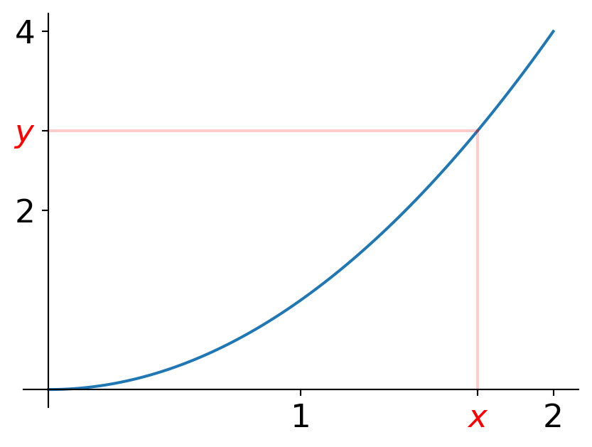
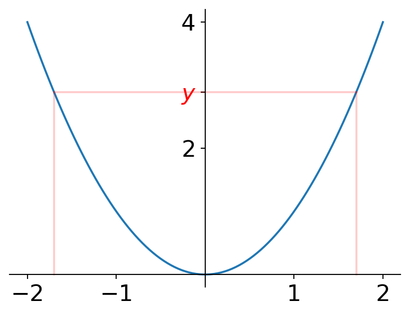
Now, the good news is that a cdf $F_X: \R \to [0,1]$ of some random variable $X$ is not just any old function, there is some structure in place: we know that it is non-decreasing, right-continuous and \[\lim_{x \to -\infty} F_X(x)=0 \quad \text{and} \quad \lim_{x \to \infty} F_X(x)=1 \tag{2.1}\] (cf. Section A.1.1). Looking at the first limit in Equation 2.1, recall that one of two things can happen:

there exists some $a \in \R$ so that $F_X(x)=0$ for all $x \in (-\infty,a]$ and $F_X(x)>0$ for all $x \in (a,\infty)$, or
$F_X(x)>0$ for all $x \in \R$, in which case $F_X(x)$ approaches but never reaches $0$ as $x \to -\infty$

and similarly for the second limit in Equation 2.1 it’s one of:

there exists some $b \in \R$ so that $F_X(x)=1$ for all $x \in [b,\infty)$ and $F_X(x)<1$ for all $x \in (-\infty,b)$, or
$F_X(x)<1$ for all $x \in \R$, in which case $F_X(x)$ approaches but never reaches $1$ as $x \to \infty$.

An example of case 1 (for both limits) is $X \sim \text{Unif}(0,1)$ with \[F_X(x)=\begin{cases} 0 & \text{if } x < 0 \\ x & \text{if } x \in [0,1) \\ 1 & \text{if } x \geq 1 \end{cases} \tag{2.2}\] while for instance an example where we have case 1 as $x \to -\infty$ and case 2 as $x \to \infty$ is $X \sim \text{Exp}(1)$ with \[F_X(x)=\begin{cases} 0 & \text{if } x < 0 \\ 1-e^{-x} & \text{if } x \geq 0. \end{cases} \tag{2.3}\]

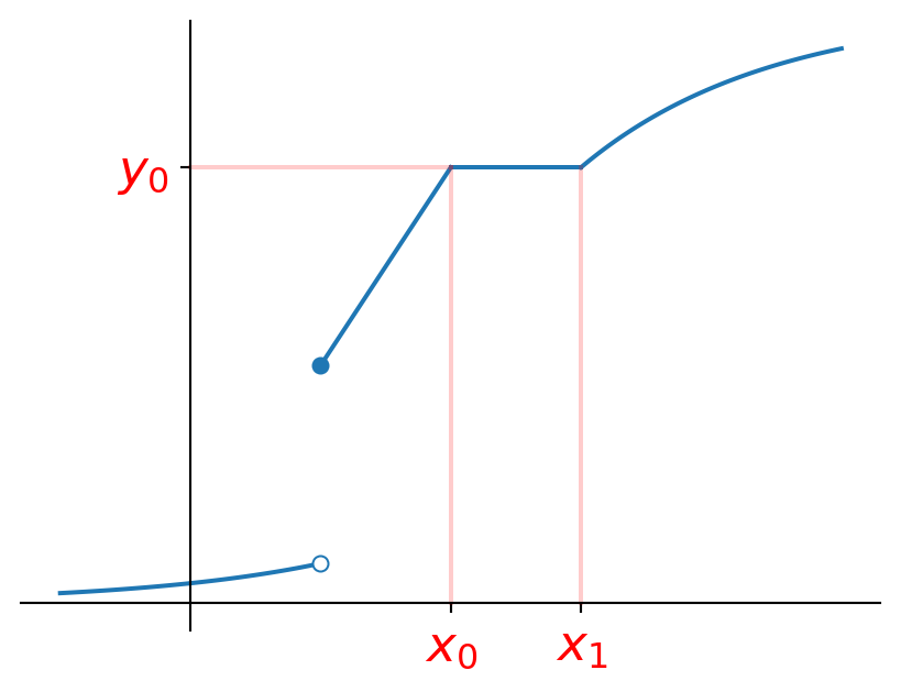
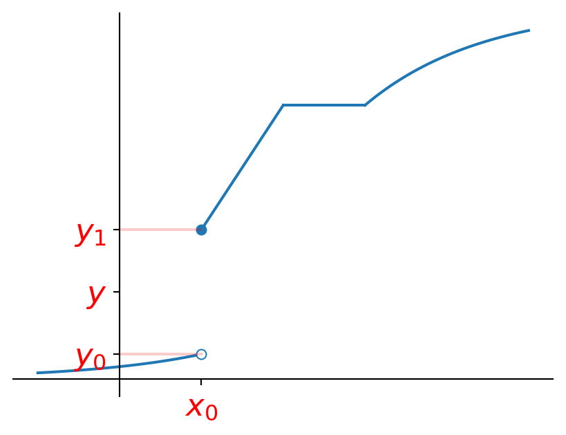
Despite that structure, a cdf is definitely not necessarily bijective. On the other hand, thanks to that structure we can easily analyse what can go wrong exactly, and we can make a sensible choice for what to do in points where the classic inverse does not exist, leading to the concept of the generalised inverse of a cdf. We focus on defining this generalised inverse for $y \in (0,1)$ only, we don’t (need to) care about $y=0$ and $y=1$ for our purposes. Effectively two things could go wrong (cf. Figure 2.2 for a visual):

$F_X$ is constant/flat on some interval $[x_0,x_1]$ i.e. for some $y_0 \in (0,1)$ it holds that $F_X(x)<y_0$ if $x<x_0$, $F_X(x)=y_0$ if $x \in [x_0,x_1]$, and $F_X(x)>y_0$ if $x >x_1$. Cf. Figure 2.2 (a). In this situation, any $x \in [x_0,x_1]$ is mapped to $y_0$ and so it’s not clear which of these should be $F_X^{-1}(y_0)$. In this case, we make the choice to set the generalised inverse equal to $x_0$. Note that this is the smallest $x$ that satisfies the inequality $F_X(x) \geq y_0$.
$F_X$ has a jump/discontinuity in some point $x_0 \in \R$, i.e. (keep in mind that $F_X$ is always right-continuous, but in this point it will fail to be left-continuous) \[y_0:=\lim_{x \uparrow x_0} F_X(x)<F_X(x_0)=:y_1.\] Cf. Figure 2.2 (b). Using that $F_X$ is non-decreasing, we have in this situation that $F_X(x) \leq y_0$ for all $x<x_0$ while $F_X(x) \geq y_1$ for all $x \geq x_0$. So in particular, $F_X$ never “visits” any $y \in (y_0,y_1)$ and its unclear what value to give $F_X^{-1}(y)$. In this case, we make the choice to set the generalised inverse equal to $x_0$. Note that this is (again!) the smallest $x$ that satisfies the inequality $F_X(x) \geq y$.

Observe that, of course, either/both cases could appear in multiple/many/… locations within the domain of $F_X$!

(a) The classic inverse of $F_X$ does not exist for $y_0$, and we **choose** to set the generalised inverse equal to $x_0$

So, the theme to deal with these problematic situation seems to be: given $y \in (0,1)$, choose $F_X^{-1}(y)$ to be the smallest $x \in \R$ that solves the inequality $F_X(x) \geq y$. In fact, as a bonus: this description also works for the classic inverse! Indeed, suppose that $F_X: \R \to [0,1]$ is a continuous and strictly increasing cdf so that it is bijective and has a classic inverse $F_X^{-1}$. Pick some $x_0 \in \R$ with $y_0:=F_X(x_0) \in (0,1)$ (again, we can safely restrict the inverse to domain $(0,1)$ for our purposes). Then, of course, $F_X^{-1}(y_0)=x_0$. To apply our theme, using that we assumed strictly increasing, we see that $F_X(x)<y_0$ resp. $F_X(x)>y_0$ for $x<x_0$ resp. $x>x_0$. So, the set of all $x$-values that satisfy $F_X(x) \geq y_0$ is simply the interval $[x_0,\infty)$ and the smallest such $x$ is indeed $x_0$!

Definition 2.1 Given a cdf $F_X: \R \to [0,1]$ of some random variable $X$, we define its generalised inverse to be the function $F_X^{-1}: (0,1) \to \R$ given by \[F_X^{-1}(y) = \inf \{ x \in \R \, | \, F_X(x) \geq y \} \quad \text{for all } y \in (0,1). \tag{2.4}\]

Some notes:

Don’t get confused, Equation 2.4 simply reads: given $y$, determine the set of all $x \in \R$ that satisfy $F_X(x) \geq y$ i.e. determine the set \[\{ x \in \R \, | \, F_X(x) \geq y \}\] and then set $F_X^{-1}(y)$ to be the infimum of this set. Recall that ‘inf’ stands for ‘infimum’, a generalisation of the minimum. It is custom to use the infimum in this definition, however in our context of applying it to a cdf this infimum is always (just) a minimum.
We use the same symbol for this generalised inverse as we normally do for the classic inverse. This makes perfect sense though, because as we argued in the paragraph above this Def: if the classic inverse exists in some point then so does the generalised inverse, and they have the same values. That is, the generalised inverse is a genuine entension of the classic inverse: it is properly defined for any cdf and where the classic inverse also exists, they coincide.
Of course, a function doesn’t care what symbol we use for its argument(s), whether it’s ‘$x$’, ‘$y$’ or even ‘Kevin’. A function is only a rule describing how its input values are processed to generate an output value. It’s appealing (I think) to use $y$ as the standard choice for inverse functions but that has no deeper meaning.
We can (of course) extend the domain of $F_X^{-1}$ to $[0,1]$ by simply applying Equation 2.4 to $y=0$ and $y=1$ as well. However this may lead to the value $\pm \infty$, for instance for the cdf $F_X$ in Equation 2.3 we would get that $F_X^{-1}(1)=\infty$. This is not some insurmountable problem, but because we won’t need it we simply don’t bother with it.

Remark 2.1. So how do you, for a given cdf $F_X$, work out its generalised inverse $F_X^{-1}: (0,1) \to \R$ explicitly? Just carry out the below for each $y \in (0,1)$:

If a unique $x \in \R$ exists so that $F_X(x)=y$, then the generalised inverse is the same as the classic inverse i.e. $F_X^{-1}(y)=x$. Typically this is the case for a whole subinterval of $(0,1)$, and then you can just use your standard tool of writing down the equation $F_X(x)=y$ and solving for $x$ to find an expression for $F_X^{-1}(y)$ covering the whole subinterval.
Otherwise you’ll need to work out Equation 2.4:
- determine the set $\{ x \in \R \, | \, F_X(x) \geq y \}$ (visually, imagine this set as part of the $x$-axis),
- find the infimum/smallest element of this set, and that is your $F_X^{-1}(y)$.

Sketching the graph of $F_X$ may be helpful to visualise stuff and see in which of these two cases each $y \in (0,1)$ goes!

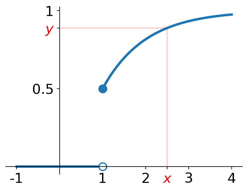
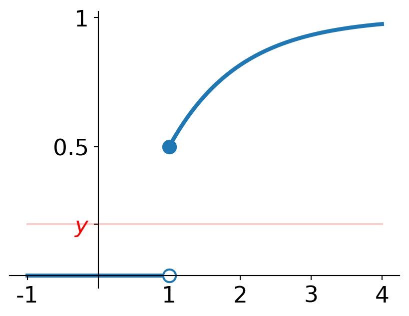
Example 2.2 To see an example of the process outlined in Remark 2.1 in action, consider e.g. the cdf $F_X$ given by \[F_X(x)=\begin{cases} 0 & \text{if } x<1 \\ 1-\frac{1}{2} e^{-(x-1)} & \text{if } x \geq 1. \end{cases} \] If you make a sketch of the graph, then it looks as in Figure 2.3 (crucial things to do: determine $F_X(1)$ by plugging $x=1$ into $1-e^{-(x-1)}/2$; check e.g. by differentiation and evaluating the limit for $x \to \infty$ what the graph of $x \mapsto 1-e^{-(x-1)}/2$ looks like).

In order to determine the generalised inverse $F_X^{-1}: (0,1) \to \R$ (recall: we only care about $y \in (0,1)$, not $y=0$ and $y=1$), we could follow the “recipe” from Remark 2.1. First observe (from your sketch or otherwise) that for any $y \in [1/2,1)$ there is a unique solution $x$ to $F_X(x)=y$ (cf. Figure 2.3 (a)). Hence for such $y$ we can just fall back to the classic inverse, and work out \[\begin{align*} F_X(x) = y &\iff 1-\frac{1}{2} e^{-(x-1)}=y \\ &\iff x=1-\log(2(1-y)) \end{align*} \tag{2.5}\] i.e. $F_X^{-1}(y)=1-\log(2(1-y))$. It remains to deal with $y \in (0,1/2)$. Fix any $y \in (0,1/2)$. Clearly (cf. Figure 2.3 (b)) there is now no solution at all to $F_X(x)=y$, and we need to go to step 2 in Remark 2.1. To determine the set $\{ x \in \R \, | \, F_X(x) \geq y \}$, we look for all $x$-values (i.e. on the horizontal axis) for which it is true that $F_X(x) \geq y$ (i.e. where the graph of $F_X$ is above or at the level $y$). You’ll hopefully agree that this holds for $x \geq 1$ (only). Hence \[\{ x \in \R \, | \, F_X(x) \geq y \}=[1,\infty).\] Now $F_X^{-1}(y)$ is the infimum of this set, so $F_X^{-1}(y)=1$ (indeed this value does not depend on which $y \in (0,1/2)$ we had exactly fixed).

In conclusion, the generalised inverse $F_X^{-1}: (0,1) \to \R$ of $F_X$ from Equation 2.5 is given by \[F_X^{-1}(y)=\begin{cases} 1 & \text{if $y \in (0,1/2)$} \\ 1-\log(2(1-y)) & \text{if $y \in [1/2,1)$.} \end{cases} \]

Finally, before we wrap up this intermezzo and go back to the inverse transform method, it will prove very convenient to write down some properties of this generalised inverse guy. For the classic inverse $f^{-1}$ of some function $f$, as you’ll remember well we have that pretty neat property that they “cancel each other out” i.e. that \[f^{-1}(f(x))=f \left( f^{-1}(x) \right)=x.\] However, as you may well had guessed, for your new friend this is no longer necessarily true. We do have the following though (if you’re interested in a proof, see e.g. Appendix 1 in McNeil, Frey, and Embrechts (2015)):

Lemma 2.1 Let $F$ be a cdf with generalised inverse $F^{-1}$ (cf. Definition 2.1). Then the following holds for all $x \in \R$ and $y \in (0,1)$:

$F^{-1}(F(x)) \leq x$; if $F$ is not constant/flat around $x$ then $F^{-1}(F(x))=x$.
$F \left( F^{-1}(y) \right) \geq y$; if $F$ is continuous in $x=F^{-1}(y)$ then $F \left( F^{-1}(y) \right)=y$.
$F(x) \geq y$ if and only if $F^{-1}(y) \leq x$.

Note:

As you’d probably have guessed, “$F$ is not constant/flat around $x$” in property i means: $F(u)<F(x)$ for all $u<x$ and $F(u)>F(x)$ for all $u>x$.

2.2.2 Formulation and proof of the inverse transform method

Good, this was all the prep we needed to do, now we can march on to stating and proving the inverse transform method for producing samples from a random variable $X$ with cdf $F_X$. We mentioned at the start of Section 2.2 already that the only condition this method requires is that we can find a “computable” expression for $F_X^{-1}$, indeed that is required in step 2 of the algorithm below:

Theorem 2.1 (Inverse transform method) Given a rv $X$ with cdf $F_X$ and its (generalised) inverse $F_X^{-1}$ (cf. Definition 2.1), a sample $x$ from $X$ can be produced as follows:

generate a sample $u$ from a $\text{Unif}(0,1)$ distribution,
set $x:=F_X^{-1}(u)$.

Proof. How do we prove that this algorithm generates samples from $X$? Well note that what actually happens is that $x$ is a sample from the random variable $Y:=F_X^{-1}(U)$, where $U \sim \text{Unif}(0,1)$. So what we need to show is that $Y$ has the same distribution as $X$, because then any sample from $Y$ is equally well a sample from $X$. Since cdf’s uniquely characterise distributions (recall from Section A.1.1 if needs be), one route to achieve this is to show that the cdf of $Y$, say $F_Y$, is the same function as $F_X$.

Before we turn to this, recall that for $U \sim \text{Unif}(0,1)$ we have that \[\P(U \leq z)=z \quad \text{for all } z \in [0,1] \tag{2.6}\] (if you had forgotten this, you could easily derive it from $U$’s pdf as listed in Appendix B e.g.).

With all this said, the proof is actually pretty straightforward! Indeed for any $v \in \R$ we have that \[\begin{align*} F_Y(v) &= \P(Y \leq v) \\ &= \P \left( F_X^{-1}(U) \leq v \right) \\ &= \P \left( F_X(v) \geq U \right) \\ &= \P \left( U \leq F_X(v) \right) \\ &= F_X(v), \end{align*} \] where the third equality uses Lemma 2.1 iii and the final one uses Equation 2.6.

Alternatively, if you don’t like the first paragraph of this proof very much/don’t find it very convincing, here is an alternative approach/phrasing. Observe that (of course!) the result of the algorithm is random. Fix some $v \in \R$. What needs to happen for the algorithm to produce a value $x$ that is less than or equal to $v$? Well we need that the $u \in (0,1)$ that is produced in step 1 of the algorithm satisfies $F_X^{-1}(u) \leq v$ i.e. by Lemma 2.1 iii that $u \leq F_X(v)$. So what is the probability that this happens? Well since $U \sim \text{Unif}(0,1)$, that is (also using Equation 2.6) $\P(U \leq F_X(v))=F_X(v)=\P(X \leq v)$. So, in conclusion, the probability that the algorithm produces a value that is less than or equal to $v$ is equal to the probability that $X$ takes a value less than or equal to $v$. Since this is true for any $v \in \R$, it is all that we need (because cdf’s i.e. such probabilities fully determine distributions, as also used above).

Let’s see a simple example of the inverse transform method in action.

Example 2.3 Here’s a toy example. Consider $X \sim \text{Exp}(1)$ with (hence) $\E[X]=1$ (cf. Appendix B if needs be). We have now two methods for producing samples from $X$: firstly it’s one of the built-in distributions in R (cf. Section 1.4.4), and secondly we could try to implement the inverse transform method from Theorem 2.1.

For the latter, we first need to try and find the inverse cdf. For this, starting with the cdf $F_X$, if you don’t know it from the top of your head you can always integrate the pdf $f_X$ (cf. Appendix B) of course: using Equation A.12 we get for any $x \in \R$ \[\begin{align*} F_X(x) &= \int_{-\infty}^x f_X(y) \d y \\ &= \begin{cases} \int_{-\infty}^x 0 \d y=0 & \text{if } x < 0 \\ \int_{0}^x e^{-y} \d y=1-e^{-x} & \text{if } x \geq 0. \end{cases} \end{align*} \] For the generalised inverse cdf $F_X^{-1}: (0,1) \to \R$, looking at Remark 2.1, if you sketch the graph of $F_X$ you’ll see that $F_X$ is a continuous function (as it should be, the cdf of a continuous random variable is always continuous after all!) and that for every $y \in (0,1)$ there is a unique $x \in (0,\infty)$ satisfying $F_X(x)=y$ (the graph has no flat/constant bits, aside from $F_X(x)=0$ for all $x \leq 0$ but we don’t care about $y=0$). So we can simply use the classic inverse here: for any $y \in (0,1)$ \[\begin{align*} y=F_X(x) &\iff y=1-e^{-x} \\ &\iff x=-\log(1-y) \end{align*} \]
i.e. $F_X^{-1}: (0,1) \to \R$ is given by $F_X^{-1}(y)=-\log(1-y)$ for all $y \in (0,1)$.

Hence the inverse transform method from Theorem 2.1 to generate a sample $x$ from $X$ takes in this situation the following form:

generate a sample $u$ from a $\text{Unif}(0,1)$ distribution,
set $x:=F_X^{-1}(u)=-\log(1-u)$.

A bit of R code to compare/contrast both methods for producing samples from $X$ is shown in Listing 2.1. Note that it uses the built-in functionality from Section 1.4.4 as well as the sapply function we saw earlier in Listing 1.4, besides the Monte Carlo simulation technique from Definition 1.1.

Listing 2.1: R code for Example 2.3

2.3 The acceptance-rejection method

Is there more to do in terms of algorithms, now we have this cute and simple inverse transform method available to us? Yes absolutely! After all that method does require that we can find the (generalised) inverse cdf, and in particular in such a form that we/the computer can efficiently compute its value for a given input (efficiently, because some kind of expression that takes long to evaluate is also of limited use of you a need a large $n$ number of samples and hence evaluations right). And this is not always possible/easy.

Take for instance a $\mathcal{N}(0,1)$ distribution, for which we don’t even have an explicit expression for its cdf, let alone the inverse cdf. Or take for instance a Beta distribution: for integer parameter values its pdf has a polynomial form (cf. Appendix B), so its cdf will also have a polynomial form, and then finding the inverse cdf boils down to finding the roots of a polynomial equation. That’s fine for first or second order, or maybe third order by a stretch, but for higher orders this quickly gets massively out of hand!

So yeah, with only the inverse transform method available we’re still quite limited in our possible applications and so it would be good to keep hunting for more. Besides a number of distribution specific algorithms – like the famous Box-Muller method (see e.g. Wiki) for the Normal distribution to mention one, another very prominent example of a general algorithm is the acceptance-rejection method.

For simplicity we formulate it for a continuous random variable $X$ with pdf $f_X$ only (though you could formulate it for discrete random variables as well if you would like). In addition to $X$, the random variable from which we want to generate samples, this algorithm requires that we choose two more bits of input:

a random variable $Y$ with pdf $f_Y$, which we call the auxiliary random variable. In principle it could be anything (as long as we can make the next bullet point work), but a practical requirement is that we can easily/efficiently produce samples from it. In our journey so far that means that it should either be a built-in distribution (cf. Section 1.4.4) or that we should be able to implement the inverse transform method (cf. Theorem 2.1) for it. Making a good/efficient choice for $Y$ is not always very obvious and mostly a matter of building up a lot of experience. In this course, we’ll always keep in mind that you don’t have that experience yet of course.
a constant $c>0$ with the property that \[c f_Y(x) \geq f_X(x) \quad \text{for all } x \in \R. \tag{2.7}\]

Remark 2.2. Just to discuss the choice of $Y$ a little bit further: Equation 2.7 sheds some light on where the difficulty with a good choice for the inputs can be. Note that any pdf integrates to $1$ over the real line, which generally (some more pathological cases excluded) means that it tends to $0$ as $x \to -\infty$ and $x \to \infty$. Looking at Equation 2.7 and assuming our pdf’s remain strictly positive for convenience, this means that we should make sure that $f_Y$ does not tend to $0$ too quickly relative to $f_X$. Indeed if it does, in particular if $f_X(x)/f_Y(x) \to \infty$ if either $x \to -\infty$ or $x \to \infty$, then it is impossible to find a constant $c>0$ satisfying Equation 2.7 because it doesn’t exist!

However, on the other hand, a choice for $Y$ that comes with an $f_Y$ that is much larger than $f_X$ in its “tails” i.e. for $x \to \pm \infty$ is also not brilliant: because both pdf’s integrate to $1$, this inevitably means that on other parts of the real line $f_Y$ that is much smaller than $f_X$, which in turn means that in order to satisfy Equation 2.7 (“for all $x \in \R$”) we are forced to choose a pretty large value of $c$. And this in turn means that on most/all of the real line, $cf_Y$ is much larger than $f_X$. As will become apparent in Theorem 2.2 below, this makes the acceptance-rejection method rather inefficient.

So, as conclusion from this very quick discussion: ideally you’d like to choose a $Y$ with an $f_Y$ that has more or less the same “tail behaviour” as $f_X$!

Here is the formulation and proof of the algorithm:

Theorem 2.2 (Acceptance-rejection method) Given a continuous random variable $X$ with pdf $f_X$ from which you would like to produce samples, choose the following:

a continuous random variable $Y$ with pdf $f_Y$ (the auxiliary random variable), and
a constant $c>0$ satisfying \[c f_Y(x) \geq f_X(x) \quad \text{for all } x \in \R. \tag{2.8}\]

Then the acceptance-rejection method for producing a sample $x$ from $X$ is the following two step algorithm:

Generate a sample $y$ from $Y$ and a sample $u$ from $U \sim \text{Unif}(0,1)$ (independent of $Y$).
1. if it holds that \[u \leq \frac{f_X(y)}{c f_Y(y)}\] then set $x:=y$ (accept),
2. otherwise, i.e. if \[u > \frac{f_X(y)}{c f_Y(y)}\] then go back to step 1 (reject).

Some notes:

Note that after executing step 1, we have real numbers $y \in \R$ and $u \in (0,1)$. Then in step 2 the algorithm tells us to work out the number $f_X(y)/(c f_Y(y))$ (just plugging the $y$ from step 1 into the given/chosen pdf’s and using the chosen value for $c$) and to compare this number with the $u$ from step 1. If that comparison brings us to case a, then we are in the “accept branch” and we get a sample $x$ from $X$ (by setting it equal to the number $y$ from step 1). However if we end up in case b rather, the “reject branch”, then no sample from $X$ is produced and we need to just try again: go back to step 1, produce new (normally different) samples $y$ and $u$ and hopefully we get more lucky this time. This hence means that, contrary to the inverse transform method from Theorem 2.1, executing one run of this algorithm is not guaranteed to produce a sample from $X$!
Obviously, the more often we end up in the “accept branch” the more efficient the algorithm is in the sense that the quicker we get to the $n$ samples from $X$ that we need for our application. Looking at the condition in case a, we see that the closer $f_X(y)/(c f_Y(y))$ is to $1$ (by non-negativity and by Equation 2.8 this ratio is always in the interval $[0,1]$) the better it is for efficiency of our algorithm. Remark 2.2 discusses this a bit further.

In practice, that means that in order to use this algorithm efficiently in a given situation, we’re looking to choose the random variable $Y$ and constant $c>0$ so that
1. $Y$ is easy to sample from (to facilitate step 1). For this we have at this point in time either the built-in distributions (cf. Section 1.4.4) or the inverse transform method (cf. Theorem 2.1) available.
2. $c f_Y$ is as small as possible on as much of the real line as possible (for the sake of efficiency), while still respecting Equation 2.8 of course.
For the purpose of this course, you’ll normally always be given/suggested a suitable $Y$ to work with. Then all that remains to be chosen is the constant $c>0$, and it follows from ii above that the best choice is the smallest $c>0$ that satifies Equation 2.8.

Proof. Assume that we have picked a continuous random variable $Y$ with pdf $f_Y$ and a constant $c>0$ so that Equation 2.8 holds. Analogue to how we did the proof of the inverse transform method (cf. Theorem 2.1), we need to prove that the (random) output of this algorithm has the same distribution as $X$. Again using that cdf’s uniquely characterise distributions (cf. Section A.1.1) it is enough to show that they have the same cdf’s, or, writing out the def of a cdf, that we have the following: \[\P(\text{output } \leq z)=\P(X \leq z) \quad \text{for all } z \in \R. \tag{2.9}\]

Fix some $z \in \R$. Note that the output of the algorithm is simply $y$, but only given that/under the condition that $u \leq f_X(y)(cf_Y(y))$ holds. So in terms of probabilities, we can write \[\P(\text{output } \leq z)=\P \left( Y \leq z \, \left| \, U \leq \frac{f_X(Y)}{cf_Y(Y)} \right. \right),\] where the random variables $Y$ and $U$ are plugged in for the samples $y$ and $u$. The rest is “just” a matter of working out this probability on the right hand side to (hopefully) see that it is equal to $\P(X \leq z)$!

We start by just working out the def of a conditional probability: \[\mathbb{P} \left( Y \leq z \, \left| \, U \leq \frac{f_X(Y)}{cf_Y(Y)} \right. \right) = \frac{\mathbb{P} \left( Y \leq z \ \& \ U \leq \frac{f_X(Y)}{cf_Y(Y)} \right)}{\mathbb{P} \left( U \leq \frac{f_X(Y)}{cf_Y(Y)} \right)}. \tag{2.10}\] Now, both probabilities in the right hand side involve two random variables: $U$ and $Y$. The good news is that they are independent (recall the statement of the theorem). You’ll remember (right? ;)) from your earlier prob courses that there are (at least) two ways forward with such probs: express them as a double integral over a suitable region in $\R^2$ of the joint cdf, or use conditioning. For the former, by independence the joint pdf is just the product of the pdf’s of $Y$ and $U$ and then it is a matter of finding the suitable regions and working out the double integrals. If you prefer that method, fine of course!

I’ll go down the conditioning route. In that method, you bring in some conditioning to give one of the two random variables a fixed value so that the resulting probability is just a prob of one random variable and hence easier to work out, and then you use the Law of Total Expectation (cf. Equation A.48 & Equation A.49) to find the original probability.

First consider \[\mathbb{P} \left( U \leq \frac{f_X(Y)}{cf_Y(Y)} \right).\] The observation here is that if $Y$ was replaced by some fixed value, then this was suddenly a very easy prob to compute! Indeed, if we define \[\psi(y):=\mathbb{P} \left( \left. U \leq \frac{f_X(Y)}{cf_Y(Y)} \right| Y=y \right) \quad \text{for all } y \in \text{Range}(Y)\] then we can easily work out \[\begin{align*} \psi(y) &= \mathbb{P} \left( \left. U \leq \frac{f_X(Y)}{cf_Y(Y)} \right| Y=y \right) \\ &= \mathbb{P} \left( U \leq \frac{f_X(y)}{cf_Y(y)} \right) \\ &= \frac{f_X(y)}{cf_Y(y)}, \end{align*} \] where the final step uses that $U \sim \text{Unif}(0,1)$ and so Equation 2.6 applies. Applying the Law of Total Expectation (cf. Equation A.48 & Equation A.49) now gives us that \[\begin{align*} \mathbb{P} \left( U \leq \frac{f_X(Y)}{cf_Y(Y)} \right) &= \E[\psi(Y)] \\ &= \int_{-\infty}^\infty \psi(y) f_Y(y) \d y \\ &= \int_{-\infty}^\infty \frac{f_X(y)}{cf_Y(y)} f_Y(y) \d y \\ &= \frac{1}{c} \int_{-\infty}^\infty f_X(y) \d y \\ &= \frac{1}{c}, \end{align*} \tag{2.11}\] where the second equality is just the integral you get if you work out the expectation of some function $\psi$ of $Y$ (cf. Equation A.16), the third plugs in the expression for $\psi$ we found above, and the final one uses that any pdf always integrates to $1$. Neat eh. :). Note that we chose to condition on $Y$ rather than $U$ above, just because that seemed the more appealing choice, but it doesn’t matter too much which one you pick.

Next consider \[\mathbb{P} \left( Y \leq z \ \& \ U \leq \frac{f_X(Y)}{cf_Y(Y)} \right),\] which we’ll attack in the same way. Defining \[\psi(y):=\mathbb{P} \left( \left. Y \leq z \ \& \ U \leq \frac{f_X(Y)}{cf_Y(Y)} \right| Y=y \right) \quad \text{for all } y \in \text{Range}(Y),\] we see that \[\psi(y)=0 \quad \text{for all } y>z\] (after all, given that $Y=y$ for some $y>z$, it is not possible/has zero probability that $Y \leq z$) while for $y \leq z$ we get \[\begin{align*} \psi(y) &= \mathbb{P} \left( \left. Y \leq z \ \& \ U \leq \frac{f_X(Y)}{cf_Y(Y)} \right| Y=y \right) \\ &= \mathbb{P} \left( U \leq \frac{f_X(y)}{cf_Y(y)} \right) \\ &= \frac{f_X(y)}{cf_Y(y)} \end{align*} \] (because, given that $Y=y$ for some $y \leq z$, $Y \leq z$ is guaranteed to happen and can therefore be dropped from the prob). Again invoking the Law of Total Expectation yields \[\begin{align*} \mathbb{P} \left( Y \leq z \ \& \ U \leq \frac{f_X(Y)}{cf_Y(Y)} \right) &= \E[\psi(Y)] \\ &= \int_{-\infty}^\infty \psi(y) f_Y(y) \d y \\ &= \int_{-\infty}^z \frac{f_X(y)}{cf_Y(y)} f_Y(y) \d y \\ &= \frac{1}{c} \int_{-\infty}^z f_X(y) \d y \\ &= \frac{1}{c} \P(X \leq z), \end{align*} \tag{2.12}\] where we used the same arguments as for the previous invokation of this Law, and for the final equality simply that integrating a pdf over some interval translates into the probability that the random variable ends up in that interval (cf. Equation A.15).

Finally then, plugging Equation 2.11 and Equation 2.12 into Equation 2.10 yields \[\begin{align*} \mathbb{P} \left( Y \leq z \, \left| \, U \leq \frac{f_X(Y)}{cf_Y(Y)} \right. \right) &= \frac{\frac{1}{c} \P(X \leq z)}{\frac{1}{c}} \\ &= \P(X \leq z), \end{align*} \] and so Equation 2.9 follows and we’re done!

We conclude with a nice example to get some feel what working with this algorithm looks like.

Example 2.4 Consider the continuous random variable $X$ with pdf \[f_X(x) = \begin{cases} \sqrt{\frac{2}{\pi}} e^{-x^2/2} & \text{if $x>0$} \\ 0 & \text{if $x \leq 0$.} \end{cases} \tag{2.13}\] This is the so-called folded Normal distribution: if you take $Z \sim \mathcal{N}(0,1)$ then $\lvert Z \rvert$ has this distribution.

Let’s see if we can implement the acceptance-rejection method from Theorem 2.2 to produce samples from this guy — note that for this one, as for Normal distributions, we can write down the integral for the cdf i.e. Equation A.12 perfectly fine but then get stuck there (there does not exist an antiderivative), so no change of getting a “computable” expression for the inverse cdf and apply the inverse transform method!

First we need to make choices for the other two inputs, namely the auxiliary random variable $Y$ and a constant $c>0$. For $Y$ we could e.g. take an $\text{Exp}(1)$ distribution, with pdf (cf. Appendix B) \[f_Y(x) = \begin{cases} e^{-x} & \text{if $x>0$} \\ 0 & \text{if $x \leq 0$.} \end{cases} \tag{2.14}\] For our constant $c>0$, recall from Theorem 2.2 (in particular also the second bullet point under “notes”) that we are looking to find the smallest $c>0$ satisfying \[cf_Y(x) \geq f_X(x) \quad \text{for all $x \in \R$.} \tag{2.15}\] Working this out a little bit, observe that for $x \leq 0$ we have $f_X(x)=f_Y(x)=0$ and hence Equation 2.15 holds no matter what $c>0$ we choose. On the other hand, for $x>0$ Equation 2.15 translates to \[c e^{-x} \geq \sqrt{\frac{2}{\pi}} e^{-x^2/2} \iff c \geq \sqrt{\frac{2}{\pi}} e^{-x^2/2+x}.\] So, if we define the function $h: (0,\infty) \to \R$ as the right hand side: \[h(x) := \sqrt{\frac{2}{\pi}} e^{-x^2/2+x} \tag{2.16}\] then we are looking for the smallest $c>0$ that satisfies \[c \geq h(x) \quad \text{for all } x>0. \tag{2.17}\]

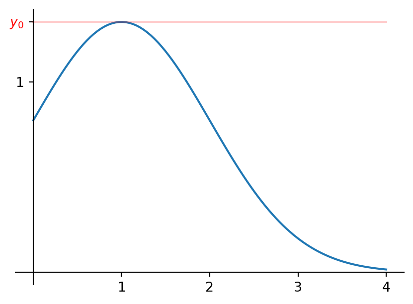
We can visualise this as follows: we are looking for the smallest/lowest vertical line $y=c$ that dominates (may touch) the graph of $h$ anywhere on $(0,\infty)$. If we define $y_0$ as the maximal value that $h$ takes, i.e. $y_0=\max_{x>0} h(x)$, then we achieve this by choosing $c=y_0$. Indeed, for any smaller value of $c$ the line $y=c$ would intersect with the graph of $h$ and (hence) not dominate it everywhere (i.e. Equation 2.17 fails to hold). For any larger value of $c$, there is some space between the line $y=c$ and the graph of $h$ and therefore a smaller (i.e. better) choice is possible. See Figure 2.4.

If you do the little bit of algebra to differentiate etc. (never forget to double check for max vs min of course!), you’ll find that $h$ attains its maximum in $x=1$, and so our choice for $c$ should be \[c=h(1)=\sqrt{\frac{2}{\pi}} e^{1/2}. \tag{2.18}\]

So, altogether, our acceptance-rejection method from Theorem 2.2 for producing samples from $X$ looks as follows:

Generate a sample $y$ from $Y$ and a sample $u$ from $U \sim \text{Unif}(0,1)$ (independent of $Y$).
1. if it holds that \[u \leq \frac{f_X(y)}{c f_Y(y)}\] then set $x:=y$,
2. otherwise, i.e. if \[u > \frac{f_X(y)}{c f_Y(y)}\] then go back to step 1

where the inputs are: $f_X$ given by Equation 2.13, $Y \sim \text{Exp}(1)$ with $f_Y$ given by Equation 2.14, and $c$ given by Equation 2.18.

Figure 2.4: A plot of $h$ from Equation 2.16

Example 2.5 Picking up Example 2.4, let’s now implement the algorithm we have already fully written down in that example. Obviously there is always about a zillion ways to do this, and whichever way you find easiest is fine of course.

In the below code, I use a structure that can easily be reused for any implementation of the acceptance-rejection algorithm (a different application only requires properly adjusting the inputs). Another aspect to consider here is that a run of the acceptance-rejection method is not guaranteed to produce a sample from $X$, and so if we want a certain number $n$ of samples, we may very well have to run the algorithm more than $n$ times. I solve that below in a very basic way: just use a loop to run the algorithm as often as is necessary to get our $n$ samples.

Further in the below code, we use the samples from $X$ to estimate $\E[X]$ using the Monte Carlo technique from Definition 1.1. And, just for fun, in this case we also know (as mentioned at the start of Example 2.4) that the random variable $\lvert Z \rvert$, where $Z \sim \mathcal{N}(0,1)$ has the same distribution as $X$. So, as an alternative route we could produce samples from $X$ by producing samples from this $\lvert Z \rvert$, which is a matter of using that the Normal distribution is built-in and that transforming samples from it by applying the absolute value function.

Listing 2.2: R code for Example 2.5

2.4 Some exercises

About the exercises

Each exercise has a (rough) indication of its difficulty, as follows:

*	easier: can be solved by (almost) only using relevant definitions/results,
**	medium: in addition to relevant definitions/results, needs a limited amount of work/creativity,
*******	harder: in addition to relevant definitions/results, needs a larger amount of work/serious creativity,
💀	warning: might make your brain hurt! These are mainly intended to provide some extra challenge for those of you keen on that and are generally quite hard. You don't need to worry about these too much for exam purposes.

The exam consists of mostly ** and *** level questions, some *, and possibly at most a few marks worth of 💀.

A bit of preaching: it is an incredibly important part of the study process to try and work on the exercises as much as possible. To become a better mathematician/learn new maths (and also to get a good exam mark ;)), above all you need to do it. And yes, of course that includes falling over things, and making mistakes, and getting stuck, and getting frustrated — all part of the game and what you’re supposed to be doing! Your lecturers have done that as well and still do it. What matters is that you don’t let that discourage you and that you make good use of the help and resources available to help you develop your skills. As part of that, many exercises have a hint in a block like this:

Hint (click to view)

Hint!

These are trying to help you on your way if you don’t know where to start or to provide some ideas if you get stuck. In spirit of the above, always have a look at these first and try again before you look at the full solution. (These hints are an extra service that won’t be available in the exam I’m afraid ;).)

Of course, we have our classes and there’s office hours, email etc. as well — I’m at any time very happy to help you with any questions you may have, and you should please never feel that any question is “too dumb” to ask!

Full/detailed solutions for the exercises will become available, just immediately below the exercises, immediately after our tutorial hour (you may have to refresh the page).

Exercise 2.1 [*/**] Suppose that $X$ is a random variable with the Rayleigh distribution (with parameter $1$), that is, with pdf \[f(x)=\begin{cases} x e^{-x^2/2} & \text{if } x>0 \\ 0 & \text{if } x \leq 0. \end{cases} \]

Find the cdf $F$ of $X$.
Write down and then implement an algorithm for producing samples from $X$. Using your algorithm, approximate $\E[X]$ and $\var(X)$.

Listing 2.3: You can do your coding here

Hint (click to view)

For i, note that $x \mapsto -e^{-x^2/2}$ is an antiderivative of $x \mapsto x e^{-x^2/2}$, and recall Equation A.12 if needs be.

For ii, to decide whether which algorithm to use, well since we have the cdf worked out we may as well try the easier inverse transform method from Theorem 2.1 no! The inverse cdf is not so hard to find – analysing your expression for $F$ a little bit(/sketching its graph) will tell you that we can just use the classic inverse (cf. the discussion in Section 2.2.1). The implementation is then a matter of reusing relevant parts from Listing 2.1 e.g. and Definition 1.1 to estimate both $\E[X]$ and $\E[X^2]$ and then estimate $\var(X)=\E[X^2]-(\E[X])^2$.

Full solution (click to view)

For i, though the pdf looks a bit scary it is actually quite easy to find an antiderivative and hence the cdf! Indeed (recall Equation A.12 if needs be) \[\begin{align*} F(x) &= \int_{-\infty}^x f(y) \d y \\ &= \begin{cases} \int_{-\infty}^x 0 \d y=0 & \text{if } x < 0 \\ \int_0^x y e^{-y^2/2} \d y = -e^{-y^2/2} \big|_{0}^x = 1-e^{-x^2/2} & \text{if } x \geq 0. \end{cases} \end{align*} \]

For ii, since we have the cdf available, we can try to make the inverse transform method (cf. Theorem 2.1) work. For this, we first need to try to find the (generalised) inverse cdf. As you can readily check (do check though!), $F$ is continuous (should be, since $X$ is continuous) with $F(0)=0$ and strictly increasing for $x \in (0,\infty)$ with $F(x) \to 1$ as $x \to \infty$ (should be as that’s true for any cdf). Make a sketch of the graph if that’s helpful, but this means that for any $y \in (0,1)$, there is a unique $x \in (0,\infty)$ that solves $F(x)=y$. So $F$ has simply a classic inverse, and we can work out for any $y \in (0,1)$ \[\begin{align*} F(x)=y &\iff y=1-e^{-x^2/2} \\ &\iff x=\sqrt{-2 \log(1-y)} \end{align*} \] (for the final step, recall from the previuous paragraph that we are looking for a solution $x \in (0,\infty)$!) i.e. $F^{-1}: (0,1) \to \R$ is given by \[F^{-1}(y)=\sqrt{-2 \log(1-y)} \quad \text{for all } y \in (0,1).\]

So we are now ready to write down the inverse transform method for producing a sample $x$ from $X$:

generate a sample $u$ from a $\text{Unif}(0,1)$ distribution,
set $x:=F^{-1}(u)=\sqrt{-2 \log(1-u)}$.

To implement this algorithm, we could just borrow lines 12–17 from Listing 2.1 e.g. Using the resulting samples to approximate $\E[X]$ and $\var(X)=\E[X^2]-(\E[X])^2$ is just a straightforward application of Definition 1.1 as we did plenty in Chapter 1:

Listing 2.4: Solution code – click “Run Code” to see the ouput

Exercise 2.2 [*/**] Suppose that we would like to produce samples from $X \sim \text{Exp}(1)$ using the acceptance-rejection method, and that we are contemplating choosing $Y \sim \text{Unif}(0,1)$ as our auxiliary random variable. Why would that be a bad choice?

Hint (click to view)

If you’re not sure, just try it and see where things go wrong! That is, start working out the algorithm (cf. Theorem 2.2) with that choice for $Y$. After writing down the pdf’s of $X$ and $Y$ (or looking them up in Appendix B), you’ll need to find the constant $c>0$. Hmmm…

Full solution (click to view)

As part of the algorithm (cf. Theorem 2.2), we need to find a $c>0$ satisfying \[c f_Y(x) \geq f_X(x) \quad \text{for all } x \in \R. \tag{2.19}\] However, after looking up the pdf’s $f_X$ and $f_Y$ in Appendix B as needs be, we see that for any $x>1$ we have $f_X(x)>0$ while $f_Y(x)=0$ and hence Equation 2.19 cannot possibly hold, for any $c>0$. This means that it is simply impossible to use this choice of $Y$.

Exercise 2.3 [**] Consider $X \sim \text{Beta}(3,4)$ (note that this distribution appears in Appendix B). Work out and write down the acceptance-rejection method for producing samples from $X$, where as auxiliary random variable we use $Y \sim \text{Unif}(0,1)$. Then implement it to approximate $\P(X>0.6)$.

Listing 2.5: You can do your coding here

Hint (click to view)

For working out the acceptance-rejection method, just follow the same steps as in Example 2.4. Then for the implementation you could first use the code from Example 2.5 (with suitably adjusted inputs) to get your hands on the samples from $X$, followed by a few lines to approximate the requested probability, for instance as in Listing 1.4.

Full solution (click to view)

Recall that the acceptance-rejection method is defined in Theorem 2.2, and that Example 2.4 is an example of how to work stuff out.

We start by writing down the pdf’s of $X$ and $Y$, for both of which we can use Appendix B if needs be: \[f_X(x)=\begin{cases} \frac{720}{12} x^2(1-x)^3 & \text{if } x \in (0,1) \\ 0 & \text{if } x \not\in (0,1), \end{cases} \tag{2.20}\] where we also used that (see the Notes at the bottom of Appendix B) \[B(3,4)=\frac{2! \cdot 3!}{6!}=\frac{12}{720},\] and \[f_Y(x)=\begin{cases} 1 & \text{if } x \in (0,1) \\ 0 & \text{if } x \not\in (0,1). \end{cases} \tag{2.21}\]

Now we need to determine the best choice for the constant $c>0$ i.e. the smallest $c>0$ so that \[cf_Y(x) \geq f_X(x) \quad \text{for all } x \in \R.\] For any $x \not\in (0,1)$, since $f_Y(x)=f_X(x)=0$, this inequality trivially holds for any choice of $c>0$ and so equivalently we can look for the smallest $c>0$ so that \[cf_Y(x) \geq f_X(x) \quad \text{for all } x \in (0,1).\] Plugging in the above expressions for $f_Y$ and $f_X$, this equivalently becomes \[c \geq \frac{720}{12} x^2(1-x)^3 \quad \text{for all } x \in (0,1).\] As also argued in Example 2.4, the smallest $c$ satisfying this condition is the maximal value of the function on the right hand side: \[c=\max_{x \in (0,1)} \frac{720}{12} x^2(1-x)^3.\] Doing the usual analysis (differentation, checking that we actually have a max (!)) you’ll find that this maximum is attained in $x=2/5$, so that we get \[c=\frac{720}{12} \left( \frac{2}{5} \right)^2 \left( \frac{3}{5} \right)^3 \approx 2.07. \tag{2.22}\]

Now we are ready to write down the acceptance-rejection method for producing a sample $x$ from this $X$, from Theorem 2.2:

Generate a sample $y$ from $Y$ and a sample $u$ from $U \sim \text{Unif}(0,1)$ (independent of $Y$).
1. if it holds that \[u \leq \frac{f_X(y)}{c f_Y(y)}\] then set $x:=y$,
2. otherwise, i.e. if \[u > \frac{f_X(y)}{c f_Y(y)}\] then go back to step 1

where the inputs are: $f_X$ given by Equation 2.20, $Y \sim \text{Unif}(0,1)$ with $f_Y$ given by Equation 2.21, and $c$ given by Equation 2.22.

Finally then, for the implementation of this algorithm, we can borrow the structure from Example 2.5 (lines 1–46 below). It then remains to use the samples from $X$ to estimate $\P(X>0.6)$, for instance using the same ideas as in Listing 1.4:

Listing 2.6: Solution code – click “Run Code” to see the ouput

You could definitely write the above code more compact, for instance using that $f_Y$ has such a simple form. However I choose here to stick as much as possible with the same structure for the sake of clarity.

Exercise 2.4 [**/***] Let $Y$ be a random variable with a so-called double exponential distribution i.e. with pdf \[f_Y(x)=\frac{\lambda}{2} e^{-\lambda \lvert x \rvert} \quad \text{for all } x \in \R,\] where $\lambda>0$ is a parameter.

Work out and write down the inverse transform method for producing samples from $Y$.
For a second random variable $X \sim \mathcal{N}(0,1)$, work out and write down the acceptance-rejection method for producing samples from $X$, where you use $Y$ as the auxiliary random variable needed in this method and find out what the best choice for its parameter $\lambda>0$ is for this purpose.

Note: if you wanted to implement the algorithm from part ii, you could follow Example 2.5 where for the sampling from $Y$ in the function get_sample_Y() you could implement the inverse transform method from part i!

Hint (click to view)

For part i, this should be a relatively straightforward working out of Theorem 2.1. Maybe the absolute value is a bit annoying, but for determining the cdf (using Equation A.12) you can just consider $x \leq 0$ and $x>0$ separately (in the latter case, split the integral into $\int_{-\infty}^0 + \int_0^x$). For the inverse cdf, analyse the cdf a bit (draw a sketch!!) and you’ll find that you can just use the classic inverse cdf (recall Section 2.2.1). To work out that inverse cdf, you could consider $y \in (0,1/2]$ and $y \in (1/2,1)$ separately.

For part ii, what makes this non-standard is that we also get to choose the parameter $\lambda>0$. Consider following a two-setp process:

first assume that $\lambda>0$ is fixed. Then we have a standard application of the algorithm, and work out what the optimal choice for $c>0$ would be in this case. Obviously this choice will depend on/be a function of $\lambda$!
now you have basically a whole range of values for $c$ you can choose from, one for every choice of $\lambda>0$. Which one would be best? Well don’t forget that, as stressed in Theorem 2.2, we’re always looking for the smallest possible value of $c>0$!

Full solution (click to view)

For part i, we’re asked to implement the method from Theorem 2.1. As in Exercise 2.1 we’ll first need to get our hands on the cdf $F_Y$ of $Y$ again, again via Equation A.12. Due to the presence of the absolute value in $f_Y$, it is a good idea to split the computation of the cdf up in negative and positive values of $x$. This gives for $x \leq 0$ \[F_Y(x)=\int_{-\infty}^x f_Y(y) \d y = \int_{-\infty}^x \frac{\lambda}{2} e^{\lambda y} \d y=\frac{1}{2}e^{\lambda x}\] while for $x>0$ \[\begin{align*} F_Y(x) &= \int_{-\infty}^x f_Y(y) \d y \\ &= \int_{-\infty}^0 \frac{\lambda}{2} e^{\lambda y} \d y + \int_0^x \frac{\lambda}{2} e^{-\lambda y} \d y \\ &= 1-\frac{1}{2} e^{-\lambda x} \end{align*} \] so altogether \[F_Y(x)=\begin{cases} \frac{1}{2}e^{\lambda x} & \text{if } x \leq 0 \\ 1-\frac{1}{2} e^{-\lambda x} & \text{if } x > 0. \end{cases} \tag{2.23}\]

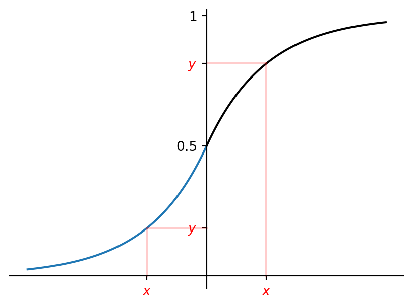
Next for the (generalised) inverse of this cdf (cf. Section 2.2.1). First we analyse $F_Y$ a bit: it is continuous (also in $0$) — as it should be, since $Y$ has a pdf and is hence a continuous random variable —, we have that $F_Y(x) \to 0$ as $x \to -\infty$ and $F_Y(x) \to 1$ as $x \to \infty$ — as it should be, that holds for any cdf — and differentiating the expressions in both cases we also easily see that $F_Y$ is strictly increasing. This means (sketch the graph!! cf. Figure 2.5) that for every $y \in (0,1)$, there is a unique $x \in \R$ solving $F_Y(x)=y$. In particular, since $F_Y(0)=1/2$, for any $y \in (0,1/2]$ the solution will be from $(-\infty,0]$ while for any $y \in (1/2,1)$ the solution will be from $(0,\infty)$.

So, $F_Y^{-1}: (0,1) \to \R$ is simply the classic inverse here, and we can find an expression by considering $y \in (0,1/2]$ and $y \in (1/2,1)$ separately. For $y \in (0,1/2]$ we get: \[\begin{align*} F_Y(x)=y &\iff y=\frac{1}{2}e^{\lambda x} \\ &\iff x=\frac{1}{\lambda} \log(2y) \end{align*} \] while for $y \in (1/2,1)$ \[\begin{align*} F_Y(x)=y &\iff y=1-\frac{1}{2} e^{-\lambda x} \\ &\iff x=\frac{-1}{\lambda} \log(2(1-y)), \end{align*} \] so altogether the inverse cdf $F_Y^{-1}: (0,1) \to \R$ is given by \[F_Y^{-1}(y)=\begin{cases} \frac{1}{\lambda} \log(2y) & \text{if } y \in (0,1/2] \\ \frac{-1}{\lambda} \log(2(1-y)) & \text{if } y \in (1/2,1). \end{cases} \tag{2.24}\]

That wraps us up, and we can now write down the inverse transform method for producing a sample $x$ from $Y$:

generate a sample $u$ from a $\text{Unif}(0,1)$ distribution,
set $x:=F_Y^{-1}(u)$, where $F_Y^{-1}$ is given by Equation 2.24.

Figure 2.5: A plot of the cdf $F_Y$ from Equation 2.23. In blue the branch/case $x \leq 0$, and in black the branch/case $x>0$

For part ii, we need to implement the acceptance-rejection method from Theorem 2.2 and we follow in principle the same steps as in Example 2.4. We know the pdf’s of $X$ (cf. Appendix B if needs be) i.e. \[f_X(x)=\frac{1}{\sqrt{2\pi}} e^{-x^2/2} \quad \text{for all } x \in \R\] and $f_Y$ as given in the question. It only remains to determine the best choice for the constant $c>0$.

The extra complication here is that we also have the freedom to choose a value for the parameter $\lambda$ appearing in the distribution of $Y$. Logically, we now follow a two-step strategy:

assuming $\lambda>0$ fixed, determine the best choice for $c>0$ (which will depend on $\lambda$!),
then look at which choice for $\lambda$ gives you the optimal value for $c>0$.

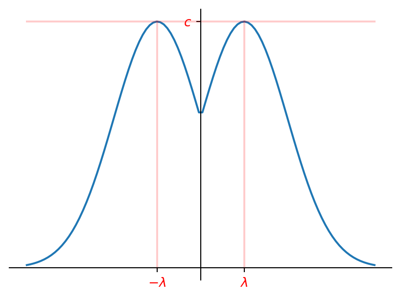
For the first step, assume $\lambda>0$ fixed for now. We know from Theorem 2.2 that the best choice for $c>0$ is the smallest $c>0$ that satisfies \[c f_Y(x) \geq f_X(x) \quad \text{for all } x \in \R\] i.e. \[c \frac{\lambda}{2} e^{-\lambda \lvert x \rvert} \geq \frac{1}{\sqrt{2\pi}} e^{-x^2/2} \quad \text{for all } x \in \R\] i.e. \[c \geq \frac{2}{\lambda \sqrt{2\pi}} e^{\lambda \lvert x \rvert -x^2/2} \quad \text{for all } x \in \R.\] As also argued in Example 2.4, the best choice i.e. the smallest $c$ is the maximal value of the right hand side i.e. \[c=\max_{x \in \R} \frac{2}{\lambda \sqrt{2\pi}} e^{\lambda \lvert x \rvert -x^2/2}.\] Denoting the function over which we want to take the maximum by $h$ and doing a bit of standard analysis using the derivative etc. (maybe you prefer to consider $x \in (-\infty,0)$ and $x \in [0,\infty)$ separately to get the absolute value out of the way) you’ll find that $h$ attains a local maximum in $x=-\lambda$ and $x=\lambda$, in which $h$ has the same value. Cf. Figure 2.6. So, in conclusion, the best choice for $c>0$ for a given, fixed $\lambda>0$ is \[c=h(-\lambda)=h(\lambda)=\frac{2}{\lambda \sqrt{2\pi}} e^{\lambda^2/2}. \tag{2.25}\]

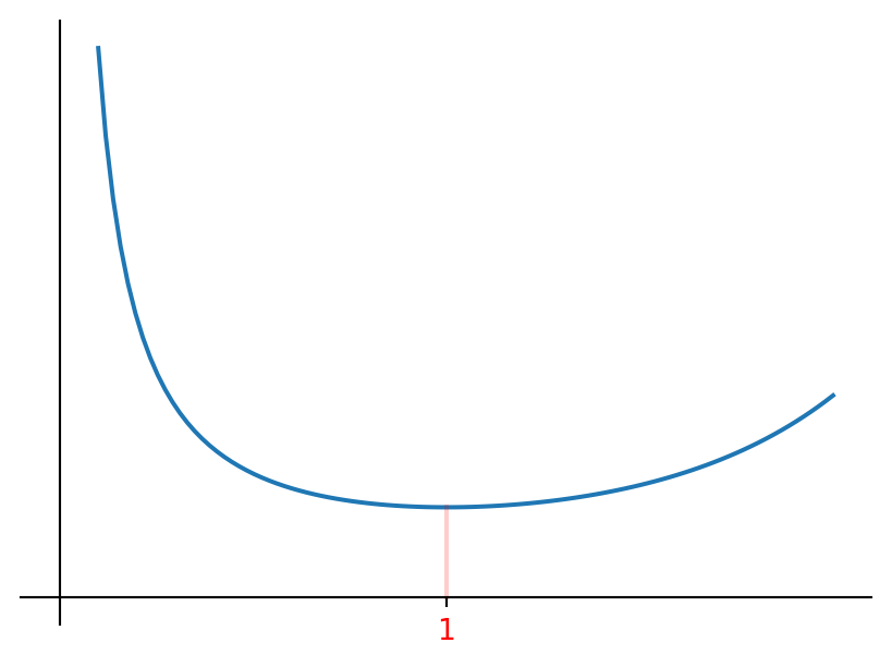
Now onto the second step: which choice of $\lambda>0$ is best? For whatever choice we make, the corresponding best choice for the constant $c$ is given by Equation 2.25, let’s denote it by $c(\lambda)$. Recall (as also used above), that our criterion is (still) to use the smallest value of $c$ that we can. So from that means that we should choose the $\lambda>0$ that minimises $c(\lambda)$. If you do a little bit of analysis (differentiation etc.), you’ll find that $c(\lambda)$ given by Equation 2.25 attains its global minimum at $\lambda=1$. Cf. Figure 2.7.

So, in conclusion, we should choose $\lambda=1$ and \[c=c(1)=\frac{2}{\sqrt{2\pi}} e^{1/2}. \tag{2.26}\] The acceptance-rejection method for producing a sample $x$ from $X$ now looks as follows. Let $Y$ have the pdf $f_Y$ as given in the question, with $\lambda=1$. For the constant $c>0$, choose Equation 2.26. Then:

Generate a sample $y$ from $Y$ and a sample $u$ from $U \sim \text{Unif}(0,1)$ (independent of $Y$).
1. if it holds that \[u \leq \frac{f_X(y)}{c f_Y(y)}\] then set $x:=y$,
2. otherwise, i.e. if \[u > \frac{f_X(y)}{c f_Y(y)}\] then go back to step 1.

Figure 2.7: A plot of the function $c(\lambda)$ for $\lambda \in (0,\infty)$

Exercise 2.5 [**] Suppose that you are managing a large project and are responsible for dealing with daily damages. From past experience you know the following. There is no damage at all for 25% of days. If there is damage during a day, then the damage amount can be modelled as an $\text{Exp}(0.01)$ distributed random variable. We denote by $X$ the damage amount on a randomly selected day.

Show that the cdf of $X$ is given by \[F(x)=\begin{cases} 1-\frac{3}{4}e^{-0.01x} & \text{if } x \geq 0 \\ 0 & \text{if } x<0. \end{cases}\]
Write down and implement the inverse transform algorithm for producing samples from $X$, and use it to estimate the expectation and variance of $X$.
Can you come up with an alternative, ad-hoc algorithm for producing samples from $X$, by simply implementing how $X$ is defined in this case i.e. by simulating what could happen on a given day and avoiding using cdf’s altogether?

Listing 2.7: You can do your coding here

Hint (click to view)

For part i, note that what the story is telling us is the following: with probability $1/4$ we have that $X=0$ while with probability $3/4$ we have that $X=Y$, where $Y \sim \text{Exp}(0.01)$. Using this info, try to work out the probability appearing in the def of the cdf i.e. $F(x)=\P(X \leq x)$ for all $x \in \R$ (cf. Equation A.4). You may find it handy to consider the cases $x<0$ and $x \geq 0$ separately.

For part ii, we’ll need to find the inverse cdf. For this, analyse $F$ a bit (make a sketch of its graph!) and observe in particular that it has a discontinuity in $x=0$. This means we’ll genuinely need the generalised inverse cdf here — get your inspiration from Example 2.2 if you’re not sure how to go about this.

For part iii, basically the question is this: if you forget about all the algorithms we have discussed (only for the moment!), and you were confronted with a random variable $X$ with the description “with probability $1/4$ we have that $X=0$ while with probability $3/4$ we have that $X=Y$, where $Y \sim \text{Exp}(0.01)$”, could you write some code that simulates this description and thereby can generate samples from $X$?

Full solution (click to view)

For part i, note that we need to work out $F(x)=\P(X \leq x)$ for all $x \in \R$ (cf. Equation A.4) and show that that results in the expression given in the question. To get some feel, observe that the question tells us that with probability $1/4$ we get that $X=0$ while with probability $3/4$ we get that $X=Y$, where $Y \sim \text{Exp}(0.01)$. This also shows that it makes sense to consider $x<0$ and $x \geq 0$ separately:

For $x<0$: clearly $X$ only takes non-negative values, so the probability that it ends up in $(-\infty,x]$ for $x<0$ is simply $0$ i.e. $F(x)=\P(X \leq x)=0$.
For $x \geq 0$: we need to wonder what the probability is that $X$ ends up in $(-\infty,x]$ for some $x \geq 0$ fixed. Using the feel mentioned above we could argue as follows. First, if $X=0$ then we are indeed in $(-\infty,x]$. Secondly, if $X=Y$ then we end up in $(-\infty,x]$ exactly if $Y$ ends up there. That is to say, we have that \[F(x)=\P(X \leq x)=\frac{1}{4}+\frac{3}{4} \P(Y \leq x). \tag{2.27}\] If you agree with this, then it’s only a matter of working this out a little bit further: since $\P(Y \leq x)=1-e^{-0.01x}$ (if you don’t remember the cdf of an $\text{Exp}(0.01)$ distribution, just derive it from its pdf (cf. Appendix B if needs be) and Equation A.4), Equation 2.27 becomes \[\begin{align*} F(x) &= \frac{1}{4}+\frac{3}{4} \left( 1-e^{-0.01x} \right) \\ &= 1-\frac{3}{4} e^{-0.01x}. \end{align*} \]

So, putting both cases together, we indeed arrive at \[F(x)=\begin{cases} 1-\frac{3}{4}e^{-0.01x} & \text{if } x \geq 0 \\ 0 & \text{if } x<0. \end{cases}\]

Note: obviously there’s a myriad of ways to do an analysis like this: using a tree diagram, using conditioning, … Whatever works best for you!

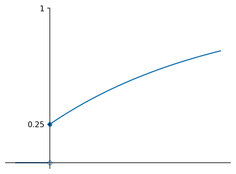
For part ii, to use the inverse transform method from Theorem 2.1, we first need the inverse cdf (cf. Section 2.2.1). As before, we start with a bit of analysis of this $F$. Obviously, if a cdf is formulated with multiple cases, we always have to be careful that there is no discontinuity hidden in that switch. And in this case there is: $F(0)=1-3/4=1/4>0$! Further for $x>0$, some differentiation shows that $F(x)$ is strictly increasing as $x$ grows, with limit $1$ as $x \to \infty$. So the graph of $F$ looks as in Figure 2.8.

We see, hence, that the classic inverse does not work (at least not everywhere) for this guy and we genuinely need the generalised inverse here! We follow the same thinking as in Example 2.2. For $y \in [1/4,1)$ there is a unique $x \geq 0$ solving $F(x)=y$, and we can find it in the usual way: \[y=1-\frac{3}{4}e^{-0.01x} \iff x=-100 \log \left( \frac{4}{3} (1-y) \right)\] i.e. \[F^{-1}(y)=-100 \log \left( \frac{4}{3} (1-y) \right).\] However for $y \in (0,1/4)$, Definition 2.1 tells us that we need to work out \[F^{-1}(y)=\inf \{ x \in \R \, | \, F(x) \geq y \}.\] We get that (have another look at Example 2.2 if you can’t see this) \[\{ x \in \R \, | \, F(x) \geq y \}=[0,\infty)\] with infimum $0$ i.e. $F^{-1}(y)=0$. Altogether we have that $F^{-1}: (0,1) \to \R$ is given by \[F^{-1}(y)=\begin{cases} 0 & \text{if } y \in (0,1/4) \\ -100 \log \left( \frac{4}{3} (1-y) \right) & \text{if } y \in [1/4,1). \end{cases} \]

Finally, with this expression for $F^{-1}$ ready, the implementation could be as follows (see e.g. Example 2.3 and Exercise 2.1):

Listing 2.8: Solution code – click “Run Code” to see the ouput

For part iii, the idea is to simply mimic in code how we are told that a sample of $X$ comes about:

with probability $1/4$, we get a value of $0$;
otherwise, i.e. with probability $3/4$, we get a sample from an $\text{Exp}(0.01)$ distribution.

One way to implement that case distinction is to use a $U \sim \text{Unif}(0,1)$: since $\P(U \leq 1/4)=1/4$ and (hence) $\P(U \geq 1/4)=3/4$ (recall Equation 2.6) we could generate a sample $u$ from $U$, and check whether $u \leq 1/4$ or not. So we could for instance do it as in Listing 2.9 or Listing 2.10 (which is a bit more efficient as it doesn’t use a loop).

Listing 2.9: Solution code – click “Run Code” to see the ouput

Listing 2.10: Solution code – click “Run Code” to see the ouput