Appendix A — A quick reminder of Probability basics

Let’s remind ourselves of a few basic facts around Probability Theory and, in particular, random variables — we’ll use them all the time in this course! We’ll do a quick and dirty overview of the key points that are important to us only. Note that for exam purposes, this material is only here to support the main content in the other chapters!

A.1 Random variables

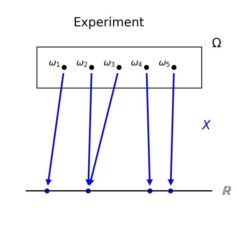
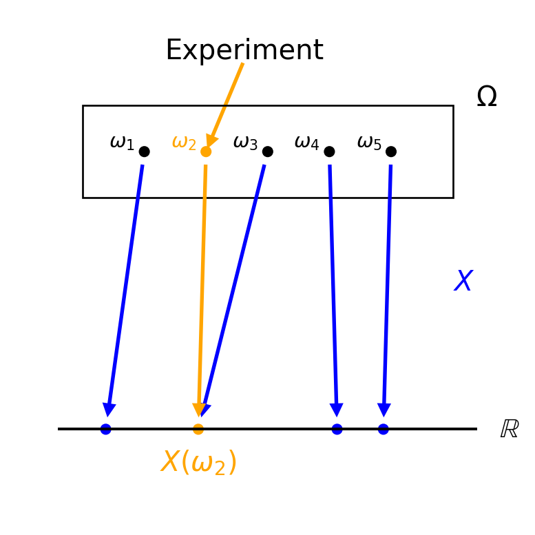
Recall from your earlier Probability courses that whenever we talk about a random variable, there is in the background always some experiment present that has a set of possible outcomes collected in a set $\Omega$. A random variable $X$ is then nothing but a mapping $X: \Omega \to \R$ that maps each possible outcome of the experiment, say $\omega \in \Omega$, to a real number $X(\omega) \in \R$.

In Probability Theory this setup is further enriched by defining events (certain, or sometimes all, subsets of $\Omega$) and by constructing a probablity measure $\P$ that assigns to each event a number from $[0,1]$ that we interpret as how likely the event is to occur (or happen) if we run the experiment once (that is, how likely is it that the outcome of the experiment we get to observe is an element of the event/subset of $\Omega$ we’re focussing on).

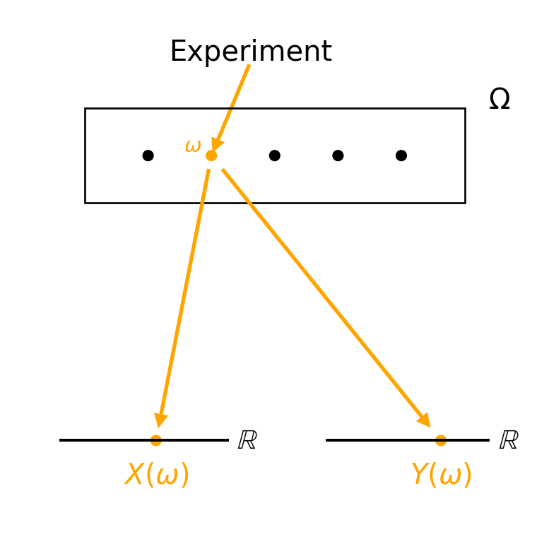
Now, each time the experiment is executed and we observe an outcome $\omega \in \Omega$, we also get to observe the corresponding value that $X$ takes: $X(\omega) \in \R$. For our purposes, we just assume that all this structure is in place to make use of the bits that we need and conveniently ignore the rest. For us, a random variable $X$ is just some random quantity we’re interested in, and each time the experiment (whatever it exactly is) is executed our random variable $X$ ends up somewhere on the real line $\R$/takes some value in $\R$. See Figure Figure A.1 for a visual.

(a) The basic setup: a random experiment whose possible outcomes (in this case five of them, generically labelled $\omega_1,\ldots,\omega_5$) are collected in $\Omega$, and a random variable $X: \Omega \to \R$ that maps each possible outcome to some real number

For example, if we do the classic experiment of rolling a fair dice and let $X$ denote the number of eyes on the dice we get to see, then each time we execute the experiment $X$ takes one of the values $1,\ldots,6$ on the real line $\R$. And we can do stuff like compute probabilities with $X$: $\P(X=1)=1/6$ (i.e. the probablity/likelihood that $X$ takes the value $1$ is $1/6$), $\P(X>4)=1/3$ (i.e. the probability/likelihood that $X$ takes a value larger than $4$ is $1/3$) etc. And of course we can compute expectations of (functions of) $X$: $\E[X]=3.5$, $\E[X^2]=91/6$ etc.

How a random variable $X$ “behaves on the real line” i.e. (roughly speaking) which values it takes and with which probabilities, is called its distribution. If $X$ and $Y$ have the same distribution i.e. the same behaviour, then all their “distributional properties” i.e. any probability, any expectation etc. are all identical i.e. for our purposes they are indistinguishable. The “well known” distributions that you have encountered in your earlier Prob courses (and a number of which are listed in Appendix B) are just specific examples that tend to pop up a lot and hence have been given a specific name.

Example A.1 Consider:

Experiment 1: a fair coin is tossed and we let $X$ count the number of Heads (so either $0$ or $1$);
Experiment 2: a fair die is rolled and we set $Y$ equal to $1$ if the number of eyes is at least $4$, and to $0$ otherwise.

Though these are very different situations, $X$ and $Y$ behave exactly the same on their real lines: $X$ takes values $0$ and $1$ with prob $1/2$ each, and $Y$ also takes values $0$ and $1$ with prob $1/2$ each. So $X$ and $Y$ have the same distribution. In particular, they both have the $\text{Bernoulli}(1/2)$ distribution (cf. Appendix B).

More mathematically, the distribution of a random variable $X$ is the following collection of probabilities¹: \[\P(X \in B) \quad \text{for all (half decent) } B \subseteq \R, \tag{A.1}\] and hence two random variables $X$ and $Y$ have the same distribution if and only if \[\P(X \in B)=\P(Y \in B) \quad \text{for all (half decent) } B \subseteq \R. \tag{A.2}\]

¹ There are some deep technicalities here, some particularly weird subsets should not be considered, but we don’t want to get into!

Finally, since a random variable $X$ is a function with codomain $\R$, we can also naturally talk about the range of $X$ i.e. the set of values in $\R$ where the random variable can actually really end up. In mathematical notation it is the set \[ \text{Range}(X)=\{ X(\omega) \, | \, \omega \in \Omega \} \subseteq \R. \tag{A.3}\] The range of the random variable $X$ in the above dice example is then $\{1,\ldots,6\}$, in the example visualised in Figure A.1 it is the set containing (the values of) these four blue points, and in Example A.1 $X$ and $Y$ both have range $\{0,1\}$.

A.1.1 Cumulative distribution function (cdf)

Every random variable $X$ gives rise to a cumulative distribution function (cdf), a function $F:\R \to [0,1]$ that maps each $x \in \R$ to the probability that $X$ takes a value in the interval $(-\infty,x]$ i.e. a value less than or equal to $x$²: \[F(x) = \P(X \leq x) \quad \text{for all } x \in \R. \tag{A.4}\] Such a cdf has the following properties:

² Note that, as always, the fact that we use $x$ as the symbol for the argument of this function is an arbitrary choice, it could equally well have been $y$ or $z$ or anything else!

$F$ is non-decreasing³,
$F$ is right-continuous⁴,
⁵ \[\lim_{x \to -\infty} F(x)=0 \quad \text{and} \quad \lim_{x \to \infty} F(x)=1. \tag{A.5}\]

³ I.e. if $y \geq x$, then $F(y) \geq F(x)$. Argument: since $(-\infty,y]$ contains $(-\infty,x]$, the prob that $X$ ends up in $(-\infty,y]$ must be at least as large as $(-\infty,x]$

⁴ I.e. for any $x \in \R$, $\lim_{h \downarrow 0} F(x+h)=F(x)$. Argument: as $h \downarrow 0$, the difference between $(-\infty,x+h]$ and $(-\infty,x]$ “converges” to the empty set $\emptyset$

⁵ Argument: $(-\infty,x]$ “converges” to the empty set $\emptyset$ as $x \to -\infty$ and to the whole of $\R$ as $x \to \infty$

The converse is also true: if $F$ is any function satisfying these three properties, then it can be shown that there exists a random variable $X$ (associated with some experiment etc.) so that $X$ has $F$ as its cdf i.e. so that Equation A.4 holds.

The reason that cdf’s play such a very central role is the following: the cdf of a random variable $X$ uniquely characterises the distribution of $X$ i.e. how $X$ “behaves on the real line” and hence any probability, expectation etc. involving $X$ (recall from Section A.1). So two random variables $X$ and $Y$ have the same distribution if and only if their cdf’s are identical i.e. (using Equation A.4) if and only if \[\P(X \leq x) = \P(Y \leq x) \quad \text{for all } x \in \R \tag{A.6}\] (comparing/contrasting with Equation A.6: apparently it is sufficient to consider only sets $B=(-\infty,x]$ in Equation A.6 rather than all $B \subseteq \R$).

The above story shows that there is a one-to-one relationship between the collection of all possible cdf’s i.e. all functions $F: \R \to [0,1]$ satisfying properties 1–3 above and the collection of all possible distributions that a random variable can have. Particularly handy: this allows us to represent the somewhat abstract concept of distribution by the much more concrete cdf (just a function!).

Example A.2 Taking again the situation from Example A.1, we had already deduced that $X$ and $Y$ there have the same distribtion. Indeed if you work out their respective cdf’s, $F_X$ and $F_Y$, then you find that they are identical: \[F_X(x)=F_Y(x)=\begin{cases} 0 & \text{if $x<0$} \\ 1/2 & \text{if $x \in [0,1)$} \\ 1 & \text{if $x \geq 1$.} \end{cases} \tag{A.7}\]

A.1.2 Discrete random variables

As you’ll remember, there are two specific types/families of random variables you have studied before in detail: discrete and continuous ones. This classification depends (only) on the distribution of the random variable.

A random variable $X$ is called discrete if its range (cf. Equation A.3) is either a finite set (like in Example A.1) or countably infinite. Recall that the latter means, loosely speaking, that the range is a set of elements that can be put in a list. For example $\{0,1,2,\ldots\}$, a random variable with a Poisson distribution has this range. Recall that $\R$, or any interval (except for the empty one and the singleton) in $\R$, is not countably infinite.

You’ll probably remember that for discrete random variables, the cdf is a piecewise constant function i.e. the graph of the function consists of horizontal line pieces at different heights — Equation A.7 is an example of such a function.

If $X$ is a discrete random variable with range say $\{x_1,x_2,\ldots,x_n\}$ (finite) resp. $\{x_1,x_2,\ldots\}$ (countable), then we define its probability mass function (pmf) as the function that assigns probabilities to the values in the range of $X$ i.e. \[f(x_i)=\P(X=x_i) \quad \text{for all } i=1,\ldots,n \quad \text{resp.} \quad \text{for all } i=1,2,\ldots. \tag{A.8}\] Further for any function $h: \R \to \R$ we can compute $\E[h(X)]$ as follows: \[\E[h(X)]=\sum_{i=1}^n h(x_i) \P(X=x_i) \quad \text{resp.} \quad \E[h(X)]=\sum_{i=1}^\infty h(x_i) \P(X=x_i). \tag{A.9}\] Note that by plugging in the identity function $h(x)=x$ we get the well known formula for the expectation of $X$ itself: \[\E[X]=\sum_{i=1}^n x_i \P(X=x_i) \quad \text{resp.} \quad \E[X]=\sum_{i=1}^\infty x_i \P(X=x_i). \tag{A.10}\] Of course, in the expressions in Equation A.9 & Equation A.10 we could have replaced the probabilities $\P(X=x_i)$ by the pmf $f(x_i)$ (cf. Equation A.8) as well. Further keep in mind that an infinite sum does not necessarily converge, and if it does it could still equal $\pm \infty$ rather than a finite number!

Finally, in Appendix B you can find some of the well known discrete distributions, for easy reference throughout the course. It lists the pmf/probabilities, mean and variance. Note that the domain of the pmf given there is necessarily equal to the range! So, for example, a random variable $X$ with a $\text{Geometric}(p)$ distribution has range $\{1,2,\ldots\}$. This can be handy to look up the range of the distributions present in that liast in case you need it and don’t know it from the top of your head!

Example A.3 Picking up the random variable $X$ from Example A.1, using Equation A.10 we can compute (with $n=2, x_1=0, x_2=1$) \[\E[X]=0 \cdot \P(X=0)+1 \cdot \P(X=1)=\frac{1}{2}\] and e.g. with $h(x)=e^x$ Equation A.9 yields \[\E[e^X]=e^0 \cdot \P(X=0)+e^1 \cdot \P(X=1)=\frac{1}{2} \left( 1+e \right).\]

If we’d do these same computations for $Y$ from Example A.1 then we’d find exactly the same results — we know that a priori because $X$ and $Y$ have the same distribution (as concluded in Example A.1) and hence any prob, any expectation etc. yields the same result!

Remark A.1. A brief word about one particularly useful example of a discrete random variable, indeed the simplest of all: the good old indicator function! Fix any event $A \subseteq \Omega$. Then its indicator function is the mapping $\mathbf{1}_A: \Omega \to \R$ given by \[\mathbf{1}_A(\omega)=\begin{cases} 1 & \text{if } \omega \in A \\ 0 & \text{if } \omega \not\in A \end{cases} \] (visualise this as in Figure A.1: draw some $A$ inside $\Omega$, and then imagine that every $\omega \in A$ gets mapped to $1$ on the real line and every $\omega \not\in A$ gets mapped to $0$ on the real line). Don’t get confused by the symbol “$\mathbf{1}_A$”, it’s just a random variable like any other, it’s just that it is a convenient symbol to use as it conveyes exactly what this random variable does.

You’ll remember that indicator functions mostly show up as building blocks in expressions for more complicated random variables, where they act as an on-off-switch if you will to express different things happening for $\omega$ in different events.

Regularly useful observation: clearly the possible values of $\mathbf{1}_A$ are $0$ and $1$ i.e. its range is $\{0,1\}$ and hence Equation A.10 yields \[\begin{align*} \E[\mathbf{1}_A] &= 0 \cdot \P(\mathbf{1}_A=0)+1 \cdot \P(\mathbf{1}_A=1) \\ &= 0 \cdot \P(A^c)+1 \cdot \P(A) \\ &= \P(A). \end{align*} \tag{A.11}\]

A.1.3 Continuous random variables

Within the random variables with a range that is not finite or countably infinite, so are not discrete random variables, we have the family of continuous random variables (the “within” here is strict: there are random variables that are neither discrete nor continuous!).

A random variable $X$ is continuous if its cdf (recall from Section A.1.1) $F_X$ has the following property: there exists a(n integrable) function $f_X: \R \to [0,\infty)$ so that \[F_X(x)=\int_{-\infty}^x f_X(y) \d y \quad \text{for all } x \in \R. \tag{A.12}\] In this situation, $f_X$ is called the probability density function (pdf) of $X$. For this property to hold, $F_X$ must be “smooth enough”: continuous and differentiable “almost everywhere”⁶.

⁶ As long as there are finitely many points where $F_X$ is not differentiable we’re still fine. More precisely, $F_X$ must be absolutely continuous, see Wiki if you’re interested

⁷ Really? Yes! Whatever value(s) you choose in such points does not affect the integral in Equation A.12 and hence it doesn’t matter. This also means that generally, pdf’s are not unique for a given continuous random variable

Further in this situation, $f_X$ can be extracted from a given $F_X$ by setting $f_X(x)=F_X'(x)$ in any $x \in \R$ where $F_X$ is differentiable, and you can give $f_X$ whatever value you want in points where $F_X$ is not differentiable⁷ and it has the property that it integrates to $1$ (let $x \to \infty$ in Equation A.12 and recall Equation A.5): \[\int_{-\infty}^\infty f_X(y) \d y=1. \tag{A.13}\]

Example A.4 The functions \[f(x)=\begin{cases} 1 & \text{if } x \in (0,1) \\ 0 & \text{if } x \not\in (0,1) \end{cases} \] and \[g(x)=\begin{cases} 1 & \text{if } x \in [0,1] \\ 0 & \text{if } x \not\in [0,1] \end{cases} \] are both equally valid choices as pdf for a $X \sim \text{Unif}(0,1)$. Indeed, this guy has cdf \[F_X(x)=\begin{cases} 0 & \text{if } x <0 \\ x & \text{if } x \in [0,1) \\ 1 & \text{if } x \geq 1 \end{cases} \] and as you can easily check, Equation A.12 holds no matter we plug in $f$ or $g$ in the role of pdf there.

Recall that continuous random variables are a lot more murky bastards than their nice and simple discrete cousins. For instance, if $X$ is a continuous random variable then it holds that \[\P(X=x)=0 \quad \text{for all } x \in \R \tag{A.14}\] so, each time we do the experiment $X$ ends up somewhere on the real line, yet if we fix any point on that real line and then wonder what the probability is that $X$ ends up in that point we get $0$… This counterintuitive behaviour is not an actual contradiction due to the uncountability of the real line.

A slightly stronger version of this that is occassionally useful:

Lemma A.1 Let $X$ and $Y$ be two independent, continuous random variables. Then $\P(X=Y)=0$.

A possible proof is via the Law of Total Expectation: for any $y \in \R$ we have that \[\begin{align*} \psi(y) &:= \P(X=Y \, | \, Y=y) \\ &= \P(X=y \, | \, Y=y) \\ &= \P(X=y) \\ &=0, \end{align*}\] using independence (cf. Section A.5) for the third equality⁸ — and Equation A.14 for the fourth. Then from Equation A.50 \[\P(X=Y)=\E[\psi(Y)]=\E[0]=0.\]

⁸ On the one hand, in these expressions we’re conditioning on an event that has probability $0$ (cf. Equation A.14), which is a problem when it comes to the definition of conditional probabilities etc. — after all writing out the def means that we would be dividing by $0$. On the other hand, you’ll have seen in your earlier Prob courses that conditioning on an event of the form $\{Y=y\}$ for a continuous rv $Y$ is a special case where the conditioning can actually still be properly defined in such a way that it all works as you would intuitively expect/like

Recall that we compute probabilities that $X$ ends up in some interval by integrating the pdf $f_X$: for any $-\infty \leq a<b \leq \infty$ we have that \[\begin{align*} \P(a<X<b) &= \P(a \leq X<b) \\ &= \P(a < X \leq b) \\ &= \P(a \leq X \leq b) \\ &= \int_a^b f_X(y) \, \d y \end{align*} \tag{A.15}\] (the fact that it doesn’t matter whether we include the boundary point(s) of the interval or not is a manifestation of Equation A.14). I.e. the probability that $X$ ends up in an interval on the real line equals the area under the graph of $f_X$ over that interval.

Further recall that for computing the expectation $\E[h(X)]$ for any⁹ function $h: \R \to \R$ we have \[\E[h(X)]=\int_{-\infty}^\infty h(x) f_X(x) \d x \tag{A.16}\] and if we choose for $h$ the identity function i.e. $h(x)=x$ then we get just the expectation of $X$ itself: \[\E[X]=\int_{-\infty}^\infty x f_X(x) \d x. \tag{A.17}\] Keep in mind that such an integral does not necessarily exist, or can be $\pm \infty$.

⁹ Well, almost any, but we ignore some intricate technicalities here

Finally a word about the range of continuous random variables. Again murky and ambiguous stuff going on here. Long story short: in the case of a continuous random variable with pdf $f_X$, our standing convention is that we are working in a setup where \[\text{Range}(X) = \{ x \in \R \, | \, f_X(x)>0 \} \tag{A.18}\] i.e. the set of possible values that $X$ can take on the real line is exactly the set of points where its pdf (whichever one we have chosen!) is strictly positive. Further for the ones listed in Appendix B, i.e. Beta, Exponential, Gamma, Normal and Uniform, we’ll always be working with the choice of pdf listed there (in other cases, we’ll specify the pdf we’re using). So, for instance, by convention (double check for yourself using Appendix B): if $X \sim \text{Unif}(a,b)$, then $X$ has as range the interval $(a,b)$; if $X \sim \text{Gamma}(\alpha,\beta)$, then $X$ has as range the interval $(0,\infty)$; etc.

A.1.4 “Other types” of random variables

In Section A.1.1 we said that any function $F: \R \to [0,1]$ satisyfing the three properties listed there is the cdf of some random variable. In Section A.1.2 we discussed how discrete random variables have a cdf that is piecewise constant, and in Section A.1.3 how continuous random variables have a cdf that is continuous and differentiable “almost everywhere”.

Ok. But seeing all that put together, we come to the following (maybe shocking for some!) discovery: it’s not very difficult to think of an example of a function $F: \R \to [0,1]$ that does satisfy the requirements to be the cdf of some random variable, but is neither piecewise constant nor continuous and differentiable “almost everywhere”. That random variable is hence neither continuous nor discrete, so it is some “other type”. And here is the big knockout: we have no tools whatsoever for such random variables! For instance, we know from earlier Probability courses how to compute expectations for discrete and continuous random variables, but for such an “other type” random variable it’s crickets…

There is (of course!) a beautiful mathematical theory covering such random variables, a Theory of Everything for random variables if you will ;). This course is not the place to explore that, you may encounter it in some different course. We will encounter such “other type” random variables, and that’s the reason for this brief section — just to acknowledge that they exist, but always in a context allowing us to compute their expectation (for instance) using Probability tools that we do already have available.

A.2 Generating functions

There exist a number of ways to represent random variables (or rather, their distribution) in terms of a function. Indeed the cdf, as extensively discussed in Section A.1.1, is one very important example. But it’s far from the only one, there is for instance also the moment generating function, the probability generating function, the Laplace transform etc. All of these do essentially the same thing: associate/map (a suitable subset of) random variables(/distributions) with/to a certain function, in an injective i.e. one-to-one fashion. The latter means that if two random variables get mapped to the same function, then they have the same distribution.

They are mostly useful for the following reasons.

If it’s hard to get a clear handle on the distribution of a random variable we’re interested in, but we can deduce what its generating function (whichever one we’re using) is, then we still have a unique identifier of this distribution (due to the injectivity property mentioned above).
Certain operations on random variables, such as adding them up, can be quite annoying to work out via their cdf’s but much easier via generating functions.
Several types of generating functions expose very useful information about the random variable/distribution it has been applied to, such as moments (in case of the moment generating function) and probabilities (in case of the probability generating function) — indeed there seems to be something of a theme here! ;).

We will in particular be using the moment generating function (mgf): for any random variable $X$, its mgf is the function $M_X: \R \to (0,\infty]$ (where $(0,\infty]:=(0,\infty) \cup \{\infty\}$) given by \[M_X(t) = \E[e^{tX}] \in (0,\infty] \quad \text{for all } t \in \R.\] Note that the random variable $e^{tX}$ is always strictly positive, and so its expectation will be strictly positive though it may well be $\infty$ for some or even all $t \not=0$. For any random variable $X$ with $M_X(t)=\infty$ for all $t \not=0$, the mgf is degenerate/useless and these are hence normally excluded from consideration when working with the mgf.

Also note that for discrete resp. continuous random variables the mgf can be worked out using Equation A.9 resp. Equation A.16, in either case with the choice $h(x)=e^{tx}$.

Here’s how the above three mentioned general points for the use of generating functions in particular apply to mgf’s:

Mgf’s can uniquely identify distributions even by comparing them on part of their domains only: for any two random variables $X, Y$, if some $a, b \in \R$ with $a<b$ exist so that $M_X(t)=M_Y(t)<\infty$ for all $t \in (a,b)$, then $X$ and $Y$ have the same distribution.
If $X$ and $Y$ are independent, then the mgf of their sum can be found by simply multiplying their mgf’s: \[\begin{align*} M_{X+Y}(t) &= \E[e^{t(X+Y)}] \\ &= \E[e^{tX}e^{tY}] \\ &= \E[e^{tX}]\E[e^{tY}] \\ &= M_X(t) M_Y(t), \end{align*} \tag{A.19}\] where the third equality uses Equation A.56.
If you have an expression for the mgf $M_X$ of a random variable $X$, and it has the property that a $h>0$ exists so that $M_X(t)<\infty$ for all $t \in (-h,h)$, then for any $k=1,2,\ldots$ the $k$-th moment of $X$ can be computed as follows: \[\E[X^k]=M_X^{(k)}(0), \tag{A.20}\] where $M_X^{(k)}$ denotes the $k$-th derivative of $M_X$.

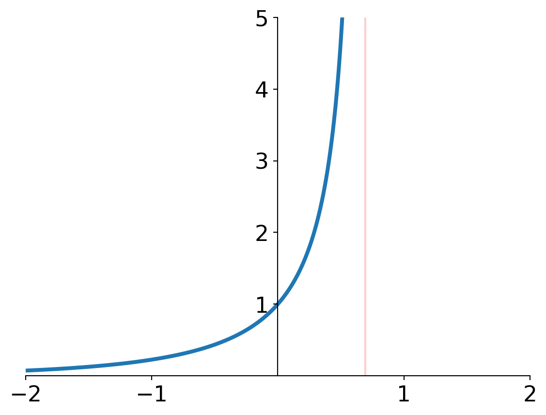
Example A.5 If $X \sim \text{Geometric}(p)$ for some $p \in (0,1)$, then \[\begin{align*} M_X(t) &= \E[e^{tX}] \\ &= \sum_{k=1}^\infty e^{tk} (1-p)^{k-1} p \\ &= \frac{p}{1-p} \sum_{k=1}^\infty \left( e^t (1-p) \right)^k \\ &= \begin{cases} \frac{p}{1-p} \left( \frac{1}{1-e^t(1-p)}-1 \right) & \text{if } e^t(1-p)<1 \\ \infty & \text{if } e^t(1-p) \geq 1 \end{cases} \\ &= \begin{cases} \frac{p e^t}{1-e^t(1-p)} & \text{if } t<\log \left( \frac{1}{1-p} \right) \\ \infty & \text{if } t \geq \log \left( \frac{1}{1-p} \right), \end{cases} \end{align*} \] where the second equality uses Equation A.9 with the choice $h(x)=e^{tx}$ and the pmf from Appendix B (if needs be), and the third the geometric series. Cf. Figure A.2 (a).

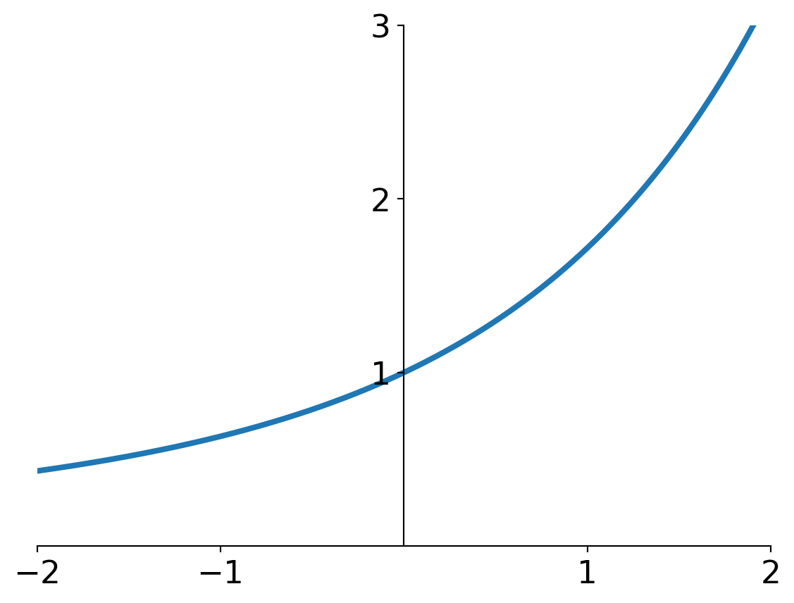
If $X \sim \text{Unif}(a,b)$ for some $a<b$, then \[\begin{align*} M_X(t) &= \E[e^{tX}] \\ &= \int_a^b e^{tx} \frac{1}{b-a} \d x \\ &= \frac{e^{tb}-e^{ta}}{t(b-a)}, \end{align*} \] where we now used Equation A.16 again with $h(x)=e^{tx}$ and the pdf from Appendix B (if needs be). Note that in this case we have $M_X(t)<\infty$ for all $t \in \R$, which wasn’t the case for the Geometric distribution. If you’re in doubt what happens for $t=0$, as we’re seemingly dividing by $0$ there: from the def it’s clear that we should always have $M_X(0)= \E[e^{t \cdot 0}] = \E[1]=1$, and that’s also how we should understand that fraction in $t=0$ (apply l’Hôpital’s rule e.g.). Cf. Figure A.2 (b).

(a) For $X \sim \text{Geometric}(1/2)$, with vertical asymptote at $t=\log(2) \approx 0.69$

A.3 Pairs/vectors of random variables

We discussed in Section A.1 that a random variable $X$ is nothing but a mapping $X: \Omega \to \R$, where the background is that an experiment is being done, one of the possible outcomes $\omega \in \Omega$ is observed, and then $X$ takes the value $X(\omega) \in \R$. Fine. But there is nothing stopping us from having multiple random variables, say $n$ of them: $X_1:\Omega \to \R$, $X_2:\Omega \to \R$, …, $X_n:\Omega \to \R$. Then the flow naturally becomes: an experiment is being done, one of the possible outcomes $\omega \in \Omega$ is observed, and then each of the random variables $X_i$ takes a value $X_i(\omega) \in \R$.

One way to think about it as follows: we have some experiment with relatively complex possible outcomes, and we want to measure $n$ different aspects/quantities of that outcome, denoted by $X_1, \ldots, X_n$. For simplicity we will focus on the case $n=2$ and write the random variables as $X$ and $Y$, but our discussion extends to $n>2$ in the obvious way.

For example, suppose that we go into the Arndale Center and randomly select somebody shopping there (the experiment) and then we measure both the length $X$ and weight $Y$ of that person. Or imagine that we roll $n$ dice (the experiment), and we could for instance be interested in the maximum number of eyes that we get to see, say $X$, as well as the sum of all the eyes say $Y$. Etc.

One new feature that comes with having multiple random variables is that they can depend on each other in interesting ways. For instance, in both examples in the previous paragraph a (relative to the experiment) large value of $X$ is likely to result in a large value for $Y$ as well (and vice versa). Part of this course is dedicated to studying such “dependency structures”.

Still focussing on $n=2$ with random variables $X$ and $Y$, we can either see them as presented above: two separate random variables each taking a value in $\R$, or equivalently (!) we can see them as put together to create a pair of random variables $(X,Y): \Omega \to \R^2$. Flow: the experiment is done, an outcome $\omega \in \Omega$ is observed, and then the pair of random variables takes the value $(X(\omega),Y(\omega)) \in \R^2$ i.e. $(X,Y)$ takes as value a point in $\R^2$, where the first coordinate is the value that $X$ takes and the second the value that $Y$ takes. The latter is typically the perspective we’ll be taking, although at moments we’ll also consider just the random variable $X$ (resp. $Y$) only i.e. temporarily ignoring the presence of $Y$ (resp. $X$). See Figure A.3 for a visual.

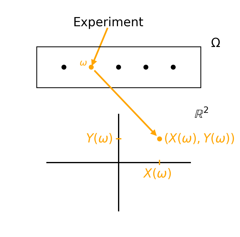
(a) We have now two random variables, $X: \Omega \to \R$ and $Y: \Omega \to \R$, who each map any $\omega \in \Omega$ to a value on their own real line. Then, when the experiment is executed and one of the possible outcomes, say the orange $\omega$, is observed, they each take a value $X(\omega)$ and $Y(\omega)$ on their real lines

Where for a single random variable we look at its “behaviour” on the real line $\R$, because that’s where it takes its values, for a pair of random variables we are then naturally interested in its “behaviour” on $\R^2$ because that’s where this guy takes its values. Many of the “behavourial” concepts for single random variables we discussed in Section A.1 have a natural analogue/extension to pairs of random variables — keeping in mind that the action stage is now $\R^2$ rather than $\R$.

For example, a pair $(X,Y)$ has a distribution, which intuitively describes how $(X,Y)$ behaves in $\R^2$ i.e. which values it takes there and with which probabilities, and which mathematically is captured by the collection of probabilities \[\P((X,Y) \in B) \quad \text{for all (half decent) } B \subseteq \R^2, \tag{A.21}\] (analogue of Equation A.1). Consequently, two pairs of random variables, $(X_1,Y_1)$ and $(X_2,Y_2)$, have the same distribution if and only if \[\P((X_1,Y_1) \in B)=\P((X_2,Y_2) \in B) \quad \text{for all (half decent) } B \subseteq \R^2. \tag{A.22}\] (analogue of Equation A.6), i.e. if for any region $B$ in the plane $\R^2$, the probability that $(X_1,Y_1)$ ends up there is the same as the probability that $(X_2,Y_2)$ ends up there. As in the univariate case (i.e. with only a single random variable), the distribution of a pair fully specifies any probability, any expectation etc., so for our purposes any two pairs with the same distrbution are effectively indistinguishable.

Further, analogue to Equation A.3, a pair $(X,Y)$ has a range which is the collection of all values in $\R^2$ where the pair can end up if the experiment is being done i.e. \[\text{Range}(X,Y)=\{ (X(\omega),Y(\omega)) \, | \, \omega \in \Omega \} \subseteq \R^2. \tag{A.23}\]

Example A.6 Let’s look at an equally simple situation as in Example A.1, but now in two dimensions:

Experiment 1: two fair coins are tossed. We let $X_1$ count the number of Heads (so either $0$ or $1$) on the first and $Y_1$ the number of Heads on the second;
Experiment 2: two fair dice are rolled. We set $X_2$ equal to $1$ if the number of eyes on the first die is at least $4$ and to $0$ otherwise, and $Y_2$ defined in the same way on the second die.

Note that both pairs, $(X_1,Y_1)$ and $(X_2,Y_2)$, have the same range, namely the collection of four points \[\{(0,0),(0,1),(1,0),(1,1)\} \tag{A.24}\] in the plane $\R^2$. Further as you can readily check \[\begin{align*} \P \big( (X_1,Y_1)=(0,0) \big) &= \P \big( (X_1,Y_1)=(0,1) \big) \\ &= \P \big( (X_1,Y_1)=(1,0) \big) \\ &= \P \big( (X_1,Y_1)=(1,1) \big) =\frac{1}{4} \end{align*} \] and also \[\begin{align*} \P \big( (X_2,Y_2)=(0,0) \big) &= \P \big( (X_2,Y_2)=(0,1) \big) \\ &= \P \big( (X_2,Y_2)=(1,0) \big) \\ &= \P \big( (X_2,Y_2)=(1,1) \big) =\frac{1}{4}. \end{align*} \]

So, $(X_1,Y_1)$ and $(X_2,Y_2)$ behave in exactly the way in $\R^2$: they take the same values with the same probabilities. Hence they have the same distribution. You could also check this conclusion more mathematically by verifying that Equation A.22 holds. It’s a bit of a job, you would have to do this by splitting all $B \subseteq \R^2$ up into a number of categories: for any $B \subseteq \R^2$ which contains none of the points from Equation A.24, we have that \[\P((X_1,Y_1) \in B)=0=\P((X_2,Y_2) \in B);\] for any $B \subseteq \R^2$ which contains one of the points from Equation A.24, we have that \[\P((X_1,Y_1) \in B)=\frac{1}{4}=\P((X_2,Y_2) \in B);\] etc.

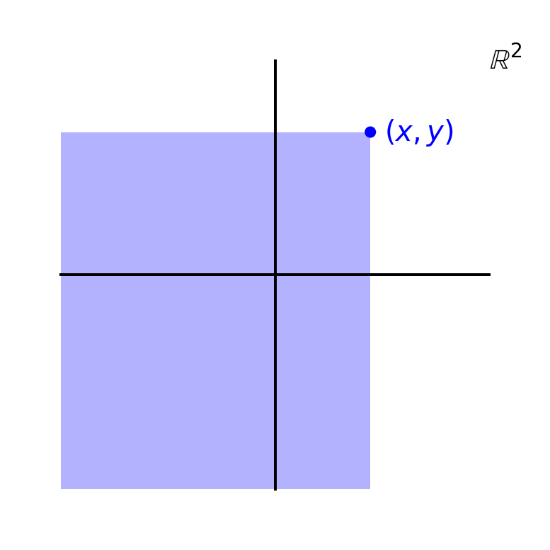
A.3.1 Joint cumulative distribution function (cdf)

Analogue to cdf’s for single random variables (cf. Section A.1.1), a pair $(X,Y)$ has a joint cumulative distribution function (joint cdf): the function $F_{X,Y}: \R^2 \to [0,1]$ given by \[F_{X,Y}(x,y)=\P(X \leq x \, \& \, Y \leq y) \quad \text{for all } x,y \in \R. \tag{A.25}\] I.e. for any $x,y \in \R$ fixed, the number $F_{X,Y}(x,y) \in [0,1]$ is the probability that $X$ takes a value not more than $x$ and that $Y$ takes a value not more than $y$ — or, equivalently, the probability that the pair $(X,Y)$ ends up somewhere in the “unbounded rectangle” in $\R^2$ which has $(x,y)$ as its upper right corner point: \[(-\infty,x] \times (-\infty,y]=\{(u,v) \, | \, u \leq x \, \& \, v \leq y \} \subseteq \R^2. \tag{A.26}\] Cf. Figure A.4 for a visual.

Figure A.4: Consider again $\R^2$ where the pair $(X,Y)$ takes its values (cf. Figure A.3 (b)). For a point $(x,y)$ in this space, $F_{X,Y}(x,y)$ is the probability that $(X,Y)$ ends up in the light blue “unbounded rectangle” Equation A.26

Analogue to cdf’s for (single) random variables (cf. Section A.1.1), it is possible to write down a list of properties such a joint cdf is guaranteed to have, and conversely that any function satisfying these properties is the joint cdf of some pair of random variables $(X,Y)$. However that is not very relevant for us so we won’t dig that all out.

Also analogue to the situation for single random variables: the joint cdf plays a central role because it uniquely characterises the distribution of the pair i.e. (roughly speaking) which values the pair takes in the plane $\R^2$ and with which probabilities, and hence any probability, expectation etc. involving the pair. In particular, the definition of two pairs $(X_1,Y_1)$ and $(X_2,Y_2)$ having the same distribution from Equation A.22 can be a bit more accessibly reformulated as that they have identical cdf’s, i.e. that \[\P(X_1 \leq x \, \& \, Y_1 \leq y)=\P(X_2 \leq x \, \& \, Y_2 \leq y) \quad \text{for all } x,y \in \R.\]

Final analogy: there is also here a one-to-one relationship between the collection of all possible joint cdf’s (i.e. all functions $F: \R^2 \to [0,1]$ satisfying the list of properties we mentioned above but were too lazy to write down) and the collection of all possible distributions that a pair of random variables can have.

Finally, let’s list some useful facts and observations about joint cdf’s.

Lemma A.2 Let $(X,Y)$ be a pair of random variables with joint cdf $F_{X,Y}$.

Observe that for a rectangle in the plane of the form \[B:= (a,b] \times (c,d]=\{ (u,v) \, | \, a<u \leq b \, \& \, c<v \leq d \} \subseteq \R^2, \tag{A.27}\] we can express the probability that $(X,Y)$ ends up in it as follows: \[\begin{align*} \P((X,Y) \in B) &= F_{X,Y}(b,d)-F_{X,Y}(a,d) \\ & \qquad -F_{X,Y}(b,c)+F_{X,Y}(a,c) \end{align*} \tag{A.28}\] You can see this visually quite easily: on the right hand side we have four probabilities for four different rectangles (each of the form as in Figure A.4 but with different upper right corner points). If you sketch these rectangles, and add/subtract them as the right hand side of Equation A.28 dictates, then indeed you’ll find that $B$ is the end result.

Further, since any half-decent $B \subseteq \R^2$ can be covered by finitely or infinitely (then in a limiting sense, e.g. for a circular $B$) many disjoint rectangles of the form Equation A.27, we can express $\P((X,Y) \in B)$ as a (possibly infinite) sum of probabilities as in Equation A.28 and hence in terms of the joint cdf! This is essentially the argument behind the claim that the distribution of a pair is uniquely characterised by its joint cdf.
In the pair $(X,Y)$, $X$ is a random variable in its own right and so is $Y$. So in particular $X$ has a distribution (on the real line), a cdf $F_X$ etc., and the same for $Y$. In this context of a pair $(X,Y)$, these are typically called the marginal distribution/cdf/… of $X$ (resp. $Y$). Since the joint cdf $F_{X,Y}$ fully characterises the distribution (its “behaviour”) of the pair, it also contains all the information about how $X$ resp. $Y$ as individual random variables behave. That is, the marginal cdf’s must somehow be “hidden” inside the joint cdf. To extract them, we can use the following: \[F_X(x)=\lim_{y \to \infty} F_{X,Y}(x,y) \quad \text{for all } x \in \R \tag{A.29}\] and \[F_Y(y)=\lim_{x \to \infty} F_{X,Y}(x,y) \quad \text{for all } y \in \R. \tag{A.30}\] The argument is (essentially) as follows: \[\begin{align*} \lim_{y \to \infty} F_{X,Y}(x,y) &= \lim_{y \to \infty} \P(X \leq x \, \& \, Y \leq y) \\ &= \P(X \leq x \, \& \, Y <\infty) \\ &= \P(X \leq x) \\ &= F_X(x), \end{align*} \] the third equality because $Y<\infty$ is trivially always true and can hence safely be removed as a condition.

Be aware though that there is no converse to this: if you know the marginal cdf’s $F_X$ and $F_Y$, then you cannot determine what the joint cdf $F_{X,Y}$ is just from that info. This is because the joint cdf hides another bit of info, namely how $X$ and $Y$ depend on each other. We’ll get to discuss this!
Although the domain of the joint cdf $F_{X,Y}$ is the whole of $\R^2$ in principle, it is sufficient (i.e. no information is lost) to take as domain only a rectangle in $\R^2$ around $\text{Range}(X,Y)$ i.e. some rectangle containing all possible values that $(X,Y)$ can take. This observation is regularly convenient when working with explicit examples, just to make the algebra a bit easier.

For example, if $X \sim \text{Unif}(0,1)$ (with range $(0,1)$) and $Y \sim \text{Unif}(0,1)$ then $\text{Range}(X,Y)$ is the unit square $(0,1)^2 \subseteq \R^2$ and we can take that (or any larger rectangle) as domain of $F_{X,Y}$. Or if $X \sim \text{Exp}(1)$ (with range $(0,\infty)$) and $Y \sim \mathcal{N}(0,1)$ (with range $\R$) then it is suffcient to consider the rectangle \[(0,\infty) \times \R=\{(x,y) \, | \, x \in (0,\infty) \text{ and } y \in \R \}\] etc. If you’re confused/not entirely sure about the ranges of $X$ and $Y$ that we used here, recall the discussion around Equation A.18!

A.3.2 Double integrals

As a brief intermezzo, let’s recall the basics of integrating functions of two variables i.e. an integral of the form \[\iint_A f(x,y) \d (x,y) \tag{A.31}\] for some (integrable) function $f: \R^2 \to \R$ and where $A \subseteq \R^2$ is the region over which we integrate. An interpretation of this integral is as follows (especially if $f$ is non-negative): take a horizontal plane where $(x,y)$ lives and add a third dimension (a $z$-axis/height if you will). The graph of $f$ i.e. all points of the form $(x,y,f(x,y))$ forms some curved plane/surface in this three dimensional space, and Equation A.31 gives the volume of the shape obtained by taking $A$ as the base/“bottom”, going straight up, and with (the relevant part of) the graph of $f$ as “top”.

For working out such an integral we can do a “single” integral twice, once over $x$ and once over $y$, and the order in which we do this does not matter. For example, if $A$ is a square in $\R^2$ i.e. \[A=[a,b] \times [c,d]=\{(x,y) \, | \, x \in [a,b] \text{ and } y \in [c,d] \}\] then \[\iint_A f(x,y) \d (x,y) = \int_a^b \int_c^d f(x,y) \d x \d y = \int_c^d \int_a^b f(x,y) \d y \d x. \tag{A.32}\] Here we read the middle integral as \[\int_a^b \left( \int_c^d f(x,y) \d x \right) \d y\] i.e. first consider $y \in [a,b]$ fixed/constant and work out the inner (“single”) integral over $x$, and then work out the outer (“single”) integral over $y$. Analogue for the rightmost integral in Equation A.32.

This principle holds no matter what shape $A$ has, it’s just that if $A$ is not a square then the bounds in the two integrals in Equation A.32 are not constant and you need to take care to get these bounds right — you’ll remember this from earlier courses and quick example below!

Example A.7 Consider the function $f: \R^2 \to \R$ given by $f(x,y)=xy^2$, and let $A$ be the triangle in $\R^2$ with vertices $(0,0)$, $(0,1)$ and $(1,0)$. Let’s compute \[\iint_A f(x,y) \d (x,y)\] by working out both the $\int \int ... \d x \d y$ and the $\int \int ... \d y \d x$ form (we claimed above that they should be equal!).

It’s all about covering your region $A$ by linepieces. These can be either horizontal or vertical.

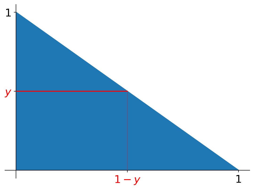
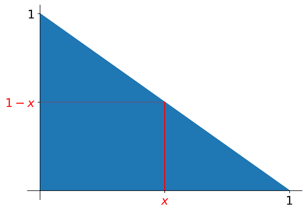
Horizontal. Take a horizontal linepiece somewhere in $A$, at a certain level $y \in [0,1]$ which we first keep fixed. This linepiece runs from $x=0$ until $x=1-y$ (as the diagonal side is the line $y=1-x$), cf. Figure A.5 (a). That means (intuitively) that this linepiece contributes \[\int_0^{1-y} f(x,y) \d x \tag{A.33}\] to the total integral. If we now consider such a line piece for every possible $y \in [0,1]$, going through them all by letting $y$ run from $y=0$ until $y=1$, then we cover the whole of $A$. Hence (intuitively) the total integral is obtained by “summing up” all the contributions of all these linepieces i.e. integrating Equation A.33 over $y$ from $y=0$ to $y=1$: \[\iint_A f(x,y) \d (x,y)=\int_0^1 \int_0^{1-y} f(x,y) \d x \d y.\]

The vertical case is analogue. Now take a vertical linepiece somewhere in $A$. This is positioned at some (fixed) $x \in [0,1]$. This linepiece runs from $y=0$ until $y=1-x$, cf. Figure A.5 (b), and therefore contributes $\int_0^{1-x} f(x,y) \d y$ to the total integral. Again covering the whole of $A$ by such linepieces, we need to let $x$ run from $0$ until $1$, and the total integral as “sum” of these contributions yields: \[\iint_A f(x,y) \d (x,y)=\int_0^1 \int_0^{1-x} f(x,y) \d y \d x. \tag{A.34}\]

Plugging in $f(x,y)=xy^2$ to get some numbers out of both these integrals (well, a number rather — should be the same!) we get that \[\begin{align*} \int_0^1 \int_0^{1-y} xy^2 \d x \d y &= \int_0^1 \left( \int_0^{1-y} xy^2 \d x \right) \d y \\ &= \int_0^1 \left( \left. \frac{x^2}{2}y^2 \right|_{x=0}^{x=1-y} \right) \d y \\ &= \int_0^1 \frac{(1-y)^2}{2} y^2 \d y \\ &= \frac{1}{60} \end{align*} \] and similarly working out Equation A.34 also yields $1/60$.

Of course, we could do somewhat less boring regions $A$ in the same way, as long as we can capture the boundary of $A$ in terms of some nice enough functions!

A.3.3 Jointly continuous pairs of random variables

In this section some double integrals appear, we briefly reviewed these in the above Section A.3.2.

A pair of random variables $(X,Y)$ is called jointly continuous if there exists a function $f_{X,Y}: \R^2 \to [0,\infty)$ (called the joint pdf) so that for any $(x,y) \in \R^2$, $F_{X,Y}(x,y)$ equals the integral of $f_{X,Y}$ over the “unbounded rectangle” in $\R^2$ with $(x,y)$ as its upper right corner point: \[A(x,y)=(-\infty,x] \times (-\infty,y] = \{ (u,v) \, | \, u \leq x \text{ and } v \leq y \} \subseteq \R^2 \tag{A.35}\] (cf. Figure A.4). That is to say¹⁰ \[F_{X,Y}(x,y) = \iint_{A(x,y)} f_{X,Y}(u,v) \d(u,v) \quad \text{for all } x,y \in \R. \tag{A.36}\] Roughly speaking this holds provided the function $F_{X,Y}$ is “smooth enough”: it must be continuous, and its mixed partial derivatives must exist “almost everywhere”¹¹ on $\R^2$.

¹⁰ Recall from Section A.3.2 that this integral can equally well be expressed as either \[\int_{-\infty}^x \int_{-\infty}^y f_{X,Y}(u,v) \d u \d v\] or \[\int_{-\infty}^y \int_{-\infty}^x f_{X,Y}(u,v) \d v \d u.\]

¹¹ Think: the points in $\R^2$ where the mixed partial derivatives fail to exist must have an area of $0$, like some curve for instance

¹² Yes, really — in the same way that in the one dimensional setting, the pdf of a continuous random variable is not unique, as discussed in Section A.1.3

If $(X,Y)$ is jointly continuous, then the joint pdf $f_{X,Y}$ can be extracted from $F_{X,Y}$ as follows: \[f_{X,Y}(x,y)=\frac{\partial^2}{\partial x \partial y} F_{X,Y}(x,y)=\frac{\partial^2}{\partial y \partial x} F_{X,Y}(x,y) \tag{A.37}\] if these mixed partial derivatives exist in $(x,y)$ (and, recall from earlier courses, then they are guaranteed to be identical) and otherwise you can choose whatever value for $f_{X,Y}(x,y)$ that you want¹². It has the property that (analogue of Equation A.13) \[\iint_{\R^2} f_{X,Y}(u,v) \d(u,v)=1.\]

The analogue of Equation A.14 is that \[\P((X,Y) \in B)=0 \tag{A.38}\] for any (half decent) set $B \subseteq \R^2$ that has (bit loosely speaking) an area of $0$. That includes a point in $\R^2$, or a finite/countable collection of points, or even a curve.

For computing probabilities (compare with Equation A.15) we have that for any (half decent) $B \subseteq \R^2$ \[\P((X,Y) \in B) = \iint_B f_{X,Y}(u,v) \d(u,v) \tag{A.39}\] (the volume of the three dimensional shape that has $B$ in the plane as its “base” and then rises straight up until it reaches the graph of $f_{X,Y}$). For computing expectations we have that for a (half decent) function $h: \R^2 \to \R$ \[\E[h(X,Y)]=\iint_{\R^2} h(u,v) f_{X,Y}(u,v) \d(u,v) \tag{A.40}\] (the two dimensional analogue of Equation A.16).

Finally we have an analogue of the discussion around Equation A.18: when we’re considering the joint pdf $f_{X,Y}$ of a pair, we will always choose things in such a way we have the following standing convention: \[\text{Range}(X,Y) = \{ (x,y) \, | \, f_{X,Y}(x,y)>0 \} \subseteq \R^2. \tag{A.41}\]

Remark A.2. Note that if $(X,Y)$ is jointly continuous, then both $X$ and $Y$ are guaranteed to be continuous random variables. However the converse is not necessarily true: if $X$ and $Y$ are continuous random variables then the pair $(X,Y)$ is not necessarily jointly continuous, it depends on the dependency structure in play!

A.4 Conditioning

In your earlier Probability courses you have already seen how important and useful the concept of conditioning is (yes you did!). This starts with the conditional probability of some event $A$ on some event $B$ with $\P(B)>0$ i.e. answering the question “How likely is it that event $A$ happens given that we know that event $B$ happens?”, naturally given by \[\P(A \, | \, B)=\frac{\P(A \cap B)}{\P(B)}. \tag{A.42}\] Indeed, for example, you’d probabily agree that the probability that the outcome of a dice roll is ⚃ given that the outcome is even equals $1/3$ (as there are three, equally likely, possible even outcomes). Indeed working this out using Equation A.42, with \[A=\{⚃\} \quad \text{and} \quad B=\{\text{outcome is even}\}=\{⚁, ⚃, ⚅\}\] we get that \[\P(A \, | \, B)=\frac{\P(A \cap B)}{\P(B)}=\frac{\P(\{⚃\})}{\P(\{⚁, ⚃, ⚅\})}=\frac{1/6}{1/2}=\frac{1}{3}.\] So, by conditioning on the extra information that the event $B$ happens, the probability that $A$ happens changes from $1/6$ (without conditioning) to $1/3$.

Now, we can do essentially the same thing with a random variable $X$. As discussed above it has a distribution i.e. it takes certain values with certain probabilities. By conditioning on an event, these probabilities will (typically) change and hence so does the distribution of $X$ as well as related quantities like the expectation of $X$. So it makes for instance sense to talk about the conditional expectation of $X$ given the event $B$, $\E[X \, | \, B]$. A general expression for it is \[\E[X \, | \, B]=\frac{\E \big[ \mathbf{1}_B X \big]}{\P(B)} \tag{A.43}\] (recall the indicator function used here from Remark A.1). Make sure to parse this expression correctly: in the numerator we take the expectation of the random variable that is the product of the two random variables $\mathbf{1}_B$ and $X$ i.e. the random variable $Y: \Omega \to \R$ given by $Y(\omega)=\mathbf{1}_B(\omega) \cdot X(\omega)$ for all $\omega \in \Omega$.

It is, with basic Prob Theory tools only, not always clear how to evaluate the numerator of Equation A.43 exactly. However in the special case that the event $B$ is an inverse image of $X$ i.e. if $B=\{X \in I\}$ for some interval (say) $I \subseteq \R$, then we can write \[\mathbf{1}_B X=\mathbf{1}_{\{X \in I\}} X=h(X)\] where $h: \R \to \R$ is the function defined as \[h(x)=\begin{cases} x & \text{if } x \in I \\ 0 & \text{if } x \not\in I \end{cases} \] and this allows us to invoke Equation A.9 in case $X$ is discrete to get \[\E \left[ \mathbf{1}_{\{X \in I\}} X \right] = \E[h(X)]=\sum_{x_i \in I} x_i \P(X=x_i) \tag{A.44}\] (where the notation in the right hand side means: sum only over those values in the range of $X$ that are contained in $I$) resp. Equation A.16 in case $X$ is continuous with pdf $f_X$ to get \[\E \left[ \mathbf{1}_{\{X \in I\}} X \right] = \E[h(X)]=\int_I x f_X(x) \d x. \tag{A.45}\]

A.4.1 Law of Total Probability/Expectation on a partition

A powerful result that quite easily follows from Equation A.42 is the Law of Total Probability (on a partition): if $B_1, B_2, \ldots, B_n$ are events that form a partition of the outcome space $\Omega$ of your experiment (i.e.: no matter what outcome your experiment will have, it is guaranteed that always exactly one of $B_1, B_2, \ldots, B_n$ will happen) with $\P(B_i)>0$ for all $i=1,\ldots,n$, then we have for any event $A$ that \[\P(A)=\sum_{i=1}^n \P(A \, | \, B_i) \P(B_i). \tag{A.46}\] This result remains true if the partition consists of infinitely many events $B_1, B_2, \ldots$. Further it remains true if one or more of the $B_i$’s has probability $0$, in that case just leave these $B_i$’s out of the summation.

A natural analogue of the law of total probability Equation A.46 is the Law of Total Expectation (on a partition) which, under the same conditions as used for Equation A.46, reads as \[\E[h(X)]=\sum_{i=1}^n \E[h(X) \, | \, B_i] \P(B_i). \tag{A.47}\]

Example A.8 Consider an experiment in which you first roll a fair dice and then you get to toss a fair coin as often as the number of eyes on your dice roll. What is the expected number of Heads you get to see?

Denoting by $X$ the number of Heads, and the partition \[B_1=\{⚀\}, B_2=\{⚁\}, \ldots, B_6=\{⚅\},\] we clearly have that $\P(B_i)=1/6$ for $i=1,\ldots,6$ and conditional on $B_i$, we get to toss the coin $i$ times and therefore the expected number of Heads in that situation is $i/2$ i.e. $\E[X \, | \, B_i]=i/2$ (I’m appaling to your intuition here, but otherwise you could resort to Equation A.43, using Equation A.44!). Plugging this into Equation A.47 yields \[\E[X]=\sum_{i=1}^6 \E[X \, | \, B_i] \P(B_i) = \sum_{i=1}^6 \frac{i}{2} \frac{1}{6}=\frac{7}{4}.\]

A.4.2 The more general Law of Total Expectation

An extension of Equation A.47 naturally arises if we consider a second random variable $Y$ in addition to $X$ and use that $Y$ for the conditioning rather than some partition. Indeed, if $Y$ is a discrete random variable with range say $\{y_1,\ldots,y_n\}$, then the results we mention below are a special case of Equation A.47 provided we use the events $\{Y=y_1\}$, $\{Y=y_2\}$, …, $\{y=y_n\}$ as our partition appearing there. However the below is truly an extension: it is valid for any random variable $Y$, in particular also if $Y$ is not discrete in which case there is no (rigorous) link with partitions anymore.

We have the following result, which is (also/still) referred to as the Law of Total Expectation (and also sometimes as the Tower Property¹³): it holds that \[\E[h(X)]=\E[\psi(Y)], \tag{A.48}\] where $\psi: \text{Range}(Y) \to \R$ is the function \[\psi(y)=\E[h(X) \, | \, Y=y] \quad \text{for all } y \in \text{Range}(Y). \tag{A.49}\] Note that the conditioning in Equation A.49 is on the event $\{Y=y\}$ i.e. the event that $Y$ takes the value $y$.

¹³ It is a special case of the more general Tower Property that involves conditioning on sigma algebras, see e.g. Wiki if you’re interested

This also works with probabilities btw: for any event $A$ \[\P(A)=\E[\psi(Y)], \tag{A.50}\] where $\psi: \text{Range}(Y) \to \R$ is the function \[\psi(y)=\P(A \, | \, Y=y) \quad \text{for all } y \in \text{Range}(Y). \tag{A.51}\]

Remark A.3. Both Equation A.48–Equation A.49 & Equation A.50–Equation A.51 remain valid if you need to compute a probability/expectation involving multiple random variables, and/or if you want to condition on multiple random variables. For instance, Equation A.48–Equation A.49 can be stretched to the following. It holds that \[\E[h(X_1,\ldots,X_n)]=\E[\psi(Y_1,\ldots,Y_m)],\] where the function $\psi: D \to \R$ is given by \[\psi(y_1,\ldots,y_m)=\E[h(X_1,\ldots,X_n) \, | \, Y_1=y_1, \ldots, Y_m=y_m] \quad \text{for all } (y_1,\ldots,y_m) \in D\] and its domain $D$ is the subset of $\R^m$ where the random vector $(Y_1,\ldots,Y_m)$ takes its values i.e. \[D=\text{Range}(Y_1) \times \text{Range}(Y_2) \times \ldots \times \text{Range}(Y_m).\]

Note that in all these laws we have written down above, Equation A.46, Equation A.47 and Equation A.48, at first glance the left hand side looks a lot simpler than the right hand side, and so it is a natural question what the point of them actually is. Well the idea is that they can be extremely powerful if you’re dealing with an event $A$ or random variable $X$ that is quite hard to understand on its own, but becomes a lot easier to understand if you could apply some (clevery chosen sometimes) conditioning. Example A.8 is a basic example of this.

Example A.9 Let’s work out Example A.8 one more time, but now using Equation A.48. For this, let $Y$ denote the number of eyes we get out of the dice roll. So \[\text{Range}(Y)=\{1,2,\ldots,6\}.\] Given that $Y=y$ i.e. that we get to see $y$ eyes, the expected number of Heads equals $y/2$, as also used in Example A.8. Using this we can work out the function $\psi$ from Equation A.49 to be \[\psi(y)=\frac{y}{2} \quad \text{for all } y \in \{1,\ldots,6\}.\] Appealing to Equation A.48, we can now find $\E[X]$ indirectly by computing $\E[\psi(Y)]$. Since this is the expectation of a function of the discrete random variable $Y$, for this we can appeal to Equation A.9: \[\E[\psi(Y)]=\sum_{y=1}^6 \psi(y) \P(Y=y) = \sum_{y=1}^6 \frac{y}{2} \frac{1}{6}=\frac{7}{4},\] so it follows from Equation A.48 that indeed $\E[X]=\E[\psi(Y)]=7/4$.

Remark A.4 (The actual power of the Law of Total Expectation). Example A.9 is nice and quick but does not really do justice to how powerful the Law of Total Expectation Equation A.48 really is (also relative to Equation A.47). That comes out much clearer if $Y$ is a continuous random variable, since then the events $\{Y=y\}$ have zero probability (as also discussed in Equation A.16) and hence we can’t produce a nice partition out of such events anymore, meaning that Equation A.47 is no longer useful. But the Law of Total Expectation still is! You’ll remember from earlier Probability courses that also in such a case, the conditional expectation $\E[X \, | \, Y=y]$ can still be well defined (after some thinking) and Equation A.48 still holds!

A.5 Independence

Recall that events $A$ and $B$ are said to be independent if it holds that \[\P(A \cap B)=\P(A)\P(B). \tag{A.52}\] Naturally and elegantly, in light of the previous Section A.4, provided that $\P(B)>0$, we immediately see from Equation A.42 that independence of $A$ and $B$ is equivalent to $\P(A \, | \, B)=\P(A)$ i.e. that the probability that $A$ happens does not change if we condition on $B$!

Similary, two random variables $X$ and $Y$ are said to be independent if any event involving only $X$ is independent of any event involving only $Y$. That is, if we take any two sets $B_1, B_2 \subseteq \R$ and consider the event that $X$ ends up in $B_1$ as well as the event that $Y$ ends up in $B_1$, i.e. $\{ X \in B_1\}$ and $\{ Y \in B_2\}$, then these two events need to be independent i.e. using Equation A.52 \[\P(X \in B_1 \ \& \ Y \in B_2)=\P(X \in B_1)\P(Y \in B_2). \tag{A.53}\] Note that we can safely ignore events with probability $0$ here: if $\P(X \in B_1)=0$ and/or $\P(Y \in B_2)=0$ then both sides of Equation A.53 are guaranteed to be $0$. So we could equivalently say: $X$ and $Y$ are independent if and only if for all $B_1, B_2 \subseteq \R$ with $\P(X \in B_1)>0$ and $\P(Y \in B_2)>0$ Equation A.53 holds.

In fact we can safely throw away even many more sets: it turns out that it is also sufficient to only consider the sets in $\R$ that are of the special form $(-\infty,x]$. That is, $X$ and $Y$ are independent if and only if \[\P(X \leq x \ \& \ Y \leq y)=\P(X \leq x)\P(Y \leq y) \quad \text{for all } x,y \in \R. \tag{A.54}\]

Further note that Equation A.54 can also be read as follows: $X$ and $Y$ are independent if and only if the joint cdf $F_{X,Y}$ (cf. Section A.3.1) is equal to the product of the cdf’s of $X$ and $Y$. In fact, this can be weakened even a bit further: the joint cdf $F_{X,Y}(x,y)$ can be expressed as the product of a function of $x$ only with a function of $y$ only, if and only if $X$ and $Y$ are independent and these two functions are then the cdf’s of $X$ and $Y$.

If the pair $(X,Y)$ is jointly continuous with joint pdf $f_{X,Y}$ (cf. Section A.3.3), then $X$ and $Y$ are independent if and only if $f_{X,Y}$ is the product of the marginal pdf’s $f_X$ and $f_Y$. Even: $X$ are independent if and only if $f_{X,Y}(x,y)$ can be expressed as the product of a function of $x$ only with one of $y$ only, and in this situation the function of $x$ resp. the function of $y$ is the marginal pdf of $X$ resp. $Y$.

Recall that if $X$ and $Y$ are independent, then: \[\var(X+Y)=\var(X)+\var(Y) \tag{A.55}\] and for any (half-decent) functions $f,g: \R \to \R$ \[\E[f(X)g(Y)]=\E[f(X)] \E[g(Y)] \tag{A.56}\] (provided all expectations exist).

A.6 Sums of random variables

If $X_1,\ldots,X_n$ are random variables, then often enough we are interested in the random variable $S$ that results from taking the sum of them: \[S=\sum_{i=1}^n X_i=X_1+\ldots+X_n.\] In general you’re mostly interested to find out what the distribution of $S$ is, given that we know the distributions of each of $X_1, \ldots, X_n$. Not always an easy question though! Below some of the key results that we know from earlier courses, all under the assumption that $X_1, \ldots, X_n$ are independent of each other.

The expectation, variance and moment generating function of $S$ (giving access to higher moments of $S$ as well as uniquely characterising the distribution of $S$, cf. Section A.2) are not very hard to compute as the sum of expectations (by the standard linearity property of the expectation operator), sum of variances (using Equation A.55) and product of mgf’s (using Equation A.19): \[\begin{multline*} \E[S]=\sum_{i=1}^n \E[X_i], \quad \var(S)=\sum_{i=1}^n \var(X_i), \\ M_S(t)=M_{X_1}(t) \cdot M_{X_2}(t) \cdot \ldots \cdot M_{X_n}(t). \end{multline*} \tag{A.57}\] Just for clarity: recall that there is a standard argument to extend a result like Equation A.55 from two to more random variables, e.g. \[\begin{align*} \var(X_1+X_2+X_3) &= \var(X_1+(X_2+X_3)) \\ &= \var(X_1) + \var(X_2+X_3) \\ &= \var(X_1) + \var(X_2)+\var(X_3), \end{align*} \tag{A.58}\] so you first consider $X_1+X_2+X_3$ as the sum of $X_1$ with $X_2+X_3$ and apply Equation A.55, and then again apply Equation A.55 to the sum $X_2+X_3$. This works for any finite number of terms.
There are some special cases that you’ll have seen before, where it has been established what distribution $S$ has, in particular where $S$ stays within the same family of distributions (recall that all distributions mentioned here are listed in Appendix B):
- if $X_i \sim \text{Binomial}(m_i,p)$ for all $i=1,\ldots,n$, then \[S \sim \text{Binomial} \left( \sum_{i=1}^n m_i, p \right).\] Note that as a special case, a $\text{Bernoulli}(p)$ distribution is identical to a $\text{Binomial}(1,p)$ distribution.
- if $X_i \sim \text{Poisson}(\lambda_i)$ for all $i=1,\ldots,n$, then \[S \sim \text{Poisson} \left( \sum_{i=1}^n \lambda_i \right).\]
- if $X_i \sim \mathcal{N}(\mu_i,\sigma_i^2)$ for all $i=1,\ldots,n$, then \[S \sim \mathcal{N} \left( \sum_{i=1}^n \mu_i, \sum_{i=1}^n \sigma_i^2 \right).\]
- if $X_i \sim \text{Gamma}(\alpha_i,\beta)$ for all $i=1,\ldots,n$, then \[S \sim \text{Gamma} \left( \sum_{i=1}^n \alpha_i, \beta \right).\] Note that as a special case, an $\text{Exp}(\lambda)$ distribution is identical to a $\text{Gamma}(1,\lambda)$ distribution.
As a last resort normally, there is the possibility of using convolutions. We formulate it for $n=2$, but it can handle a sum of $n>2$ terms in principle by working out $n-1$ convolutions¹⁴ following the same logic as in Equation A.58.
- If $X_1$ is a continuous random variable with pdf $f_{X_1}$, then the cdf $F_S$ of $S=X_1+X_2$ can be found as follows: \[F_S(x)=\int_{-\infty}^\infty F_{X_2}(x-y) f_{X_1}(y) \d y \quad \text{for all } x \in \R,\] where $F_{X_2}$ is the cdf of $X_2$.
- If $X_1$ and $X_2$ are both continuous with pdf’s $f_{X_1}$ and $f_{X_2}$ resp., then $S$ is also continuous with pdf $f_S$ given by \[f_S(x)=\int_{-\infty}^\infty f_{X_1}(x-y) f_{X_2}(y) \d y \quad \text{for all } x \in \R.\]

¹⁴ Not saying it is a pleasant or quick exercise! ;)

A.7 The Law of Large Numbers and the Central Limit Theorem

Let $X_1, X_2, \ldots$ be a sequence of i.i.d. (recall: independent and identically distributed) random variables with common expectation $\mu=\E[X_i]$ and common variance $\sigma^2=\var(X_i)$ (both assumed to be well defined and finite). For any $n \geq 1$, let $S_n$ be the sum of the first $n$ of them: \[S_n = \sum_{i=1}^n X_i \tag{A.59}\]

Then the (strong) Law of Large Numbers (LLN) states that \[\P \left( \lim_{n \to \infty} \frac{S_n}{n} = \mu \right)=1. \tag{A.60}\]

The way to read this is as follows. Imagine that we do some experiment and that rather than a single (or two) random variables we have an infinite sequence of them. For instance, imagine that we have a (magical!) hand holding infinitely many dice and that we roll these all at the same time, and that we set $X_i$ to be the number of eyes on the $i$-th dice. So: when we do the experiment, all of $X_1, X_2, \ldots$ take a value. Note that for each $n \geq 1$, $S_n$ is also a random variable — in this case it is sum of the nr of eyes on the first $n$ dice. All of $S_1, S_2, \ldots$ hence also take a value once we execute the experiment, and form a sequence of numbers. Clearly $S_n$ is always at least $1$ more than $S_{n-1}$, and so the sequence of numbers $S_1, S_2, \ldots$ will get ever larger as we walk through the sequence, tending to $\infty$ as $n \to \infty$. Now Equation A.60 tells us that if we divide by $n$ i.e. we rather look at the sequence of numbers $S_1, S_2/2, S_3/3, \ldots$ then this sequence does have a limit, namely $\mu$ which is $3.5$ in this case.

Well, Equation A.60 tells us that we end up with this limit of $\mu=3.5$ with probability $1$. This is a subtle point and I don’t want to dwell on it too much — it comes as a consequence of the dark magic that is uncountability (similar to the weirdness around Equation A.16), think about it as that this limit is almost guaranteed to show up.

The Central Limit Theorem (CLT) is (even) more surprising and is maybe the most majestic result in (basic) Probablity Theory. It tells us what the distribution of the random variable $S_n$ from Equation A.59 is in the limit for $n \to \infty$: \[\lim_{n \to \infty} \P \left( \frac{S_n-\E[S_n]}{\sqrt{\var(S_n)}} \leq x \right)=\Phi(x) \quad \text{for all } x \in \R, \tag{A.61}\] where $\Phi$ is the cdf of a $\mathcal{N}(0,1)$ distribution. Of course, it follows from our i.i.d. assumption on the $X_i$’s and Equation A.57 that \[\E[S_n]=n \E[X_i]=n \mu \quad \text{and} \quad \var(S_n)=n \var(X_i)=n \sigma^2, \tag{A.62}\] so you could sub these into Equation A.61 if you prefer.

Of course, in practical applications we typically do not have an actual infinite number of random variables but rather a (very) large number of them. In such cases we rather like to use the CLT as motivation for the following approximation: \[\text{for (very) large } n: \quad \P \left( \frac{S_n-\E[S_n]}{\sqrt{\var(S_n)}} \leq x \right) \approx \Phi(x) \quad \text{for all } x \in \R. \tag{A.63}\] This of course a little bit hand wavy: how good is that approximation actually i.e. how large is the error that we are making here, and/or how large should $n$ be exactly if we want to be sure that the error is not larger than whatever we deem acceptable for the situation at hand?? It is beyond the scope of our course, but (of course!) mathematicians have worked on obtaining error bounds, and a famous such result is the Berry–Esseen theorem.

Finally, to see how the CLT ties in with (and extends) what the LLN tells us, if we let $Z \sim \mathcal{N}(0,1)$ then for (very) large $n$, Equation A.63 tells us that the random variables¹⁵ \[\frac{S_n-\E[S_n]}{\sqrt{\var(S_n)}} \quad \text{and} \quad Z\] have (approximately) the same cdf and hence (approximately) the same distribution (recall from Section A.1.1 that cdf’s uniquely determine distributions). Using Equation A.62, this means that $S_n$ has (approximately) the same distribution as $\sqrt{n \sigma^2}Z+n\mu$ i.e. (using the well known rules for linear transformations of Normal distributions) a $\mathcal{N}(n\mu,n\sigma^2)$ distribution.

¹⁵ Observe that $\E[S_n]$ and $\sqrt{\var(S_n)}$ are just constants/numbers, so this expression is the random variable $S_n$ to which a straightforward transformation (“normalisation”) is applied

This shows that both the mean and variance of $S_n$ just keep growing as $n$ increases, as you’d expect of course, but also that if we try to battle that growth a bit by dividing by $n$ i.e. we look at $S_n/n$ then this is approximately $\mathcal{N}(\mu,\sigma^2/\sqrt{n})$ distributed. Note that the variance of this guy decreases to $0$ as $n$ grows, i.e. it is for large $n$ very concentrated around its mean $\mu$. To illustrate this, using the well known properties of a Normal distribution, with probability (approx) $68.2\%$, $S_n/n$ takes its value in the interval \[\left[\mu-\frac{\sigma^2}{\sqrt{n}},\mu+\frac{\sigma^2}{\sqrt{n}} \right]\] which as $n$ grows becomes an ever more narrow interval around $\mu$!

Remark A.5 (The magic of the CLT). There is something extremely remarkable about the CLT: the limiting distribution is Normal, no matter what the common distribution of the $X_i$’s is! This is all kinds of disturbing really: firstly there is a prori no reason for there to be a limit at all, and secondly even less of a reason for that limit to be completely independent of the input! It also underlines just how special the Normal distribution is — it is somehow, out of all the possible distributions out there, the chosen one to pop up as the limit in the CLT!

Having said that, in the approximation Equation A.63 for finite $n$ you can see an influence of the common distribution of the $X_i$’s. A bit loosely speaking, in general, the more the common distribution of the $X_i$’s “resembles” a Normal distrbution, the more accurate the approximation for a given $n$ is. As extreme case, note that if the common distribution of the $X_i$’s is Normal, then as you can readily check the approximation in Equation A.63 is an actual equality, for any $n \geq 1$. What “resembles” here exactly means requires some further digging that we don’t want to get into, but one nice visual way think about it is, in the continuous case, how much the common pdf of the $X_i$’s looks similar to the famous bell shape of the Normal pdf.

Finally, as a brief comment: given how powerful and incredibly useful the CLT is, one natural question is whether it is really only limited to the case that the $X_i$’s are i.i.d., or whether we can maybe weaken that assumption somewhat so that we can apply it in more situations. Indeed this question has been researched intensely, if you’re interested in some results see e.g. Wiki.

A.8 Chebyshev’s inequality

Chebyshev’s inequality is fundamental in Probability Theory. It is the following statement: if $Z$ is a random variable with mean $\mu_Z$ and (non-zero, finite) variance $\sigma_Z^2$, then for any $z>0$ we have that \[\P(\lvert Z-\mu_Z \rvert \geq z \sigma_Z^2) \leq \frac{1}{z^2}.\] What makes it so remarkable is that it gives a bound on how far away $Z$ can be from its mean, irrespective of what distribution $Z$ has!

For example, if we plug in $z=2$ then it reads as \[\P(\lvert Z-\mu_Z \rvert \geq 2 \sigma_Z^2) \leq \frac{1}{4}, \tag{A.64}\] that is: the probability that $Z$ takes a value at least $2 \sigma_Z^2$ away from $\mu_Z$ i.e. outside the interval $(\mu_Z-2 \sigma_Z^2,\mu_Z+2 \sigma_Z^2)$ is at most $1/4$. If we take for instance $Z \sim \text{Exp}(1)$, a random variable with range $(0,\infty)$ as you know well and with $\mu_Z=\sigma_Z=1$ (see e.g. Appendix B if you’re not sure), then Equation A.64 tells us that \[\P(\lvert Z-1 \rvert \geq 2) = \P(Z \in (-1,3)) \leq \frac{1}{4}\] i.e. that with a probability of at least $3/4$, $Z$ will take a value inside the interval $(-1,3)$ rather than elsewhere in its range $(0,\infty)$. Or, put differently: if we produce a sample $z$ from $Z$, then with probability at least $3/4$ we will have that $z \in (-1,3)$. For a compare and contrast, of course we can easily compute the exact probability that $Z$ will take a value inside the interval $(-1,3)$ as, with $f_Z$ the pdf of $Z$ that we can pick up from Appendix B if needed \[\begin{align*} \P(Z \in (-1,3)) &= \int_{-1}^3 f_Z(x) \d x \\ &= \int_0^3 e^{-x} \d x \\ &= 1-e^{-3} \approx 0.95. \end{align*}\] So the exact probability is larger than the lowerbound of $3/4$ that Chebyshev’s inequality guarantees, as it should be of course. You may argue that it is quite a bit larger than $3/4$, but then I’d counter by again insisting how powerful it is that Chebyshev’s inequality gives us a bound that holds no matter what distribution $Z$ has!