5 Copulas 3: measures of dependence

So where are we at? In Chapter 3 we have discussed the basics: the definition of copula as a mathemtical object representing a dependency structure in a pair of random variables $(X,Y)$, and we have explored how all the key ingredients (distribution, joint cdf, marginal cfd’s, copula) exactly interact with each other (recall the epic² visual Equation 3.9). Then in Chapter 4 we have devised a simple to use procedure for generating new copulas/dependency structures, and did some interesting visually inspecting of scatterplots to explore the effect of using different copulas a bit.

In this final chapter on the topic, let’s get to know these dependency structures/copulas a bit more intimately then we have so far been able to, taking it beyond visual inspections of scatterplots!

5.1 What is a “measure of dependence”?

Basically the question is this: given some pair $(X,Y)$ with dependency structure/copula $C$, what can we practically say about $X$ and $Y$ interact with each other — i.e. given that $X$ does (something), what does that mean for $Y$? For instance in the case of an investor, if stock 1 modelled by $X$ has a good day, what does that mean for stock 2 modelled by $Y$?

The sad truth is that despite all the hard work we’ve done so far, we seemingly haven’t yet come much closer to answering such a question. It is not at all apparent how we (systematically) could go from having some copula expression $C(u,v)= \, ...$ specified to addressing such a question. We have to consider this while firmly keeping in mind that (non-trivial) dependency structures/copulas are intrinsically quite complicated objects that are not very easy to fully understand so there are no simple/easy/single answers here — our relationship status with copulas is best described as “it’s complicated”! ;).

So how do we make sense of complicated objects in real life? Suppose for instance that you would be looking to buy a house. Houses are rather complicated objects, there are so many factors involved. How do you get to know a house well enough to make a decision? Well you look at all the aspects that are important to you. How much does it cost? How many rooms does it have? How do you rate the area it’s in? Etc. You measure i.e. give a value to these aspects, and then the collection of measured values gives you some concrete numbers to work with rather than that complicated house itself, also to compare different houses with each other for instance.

If we focus on the aspect “price” for instance, then what you end up doing is creating a list of all houses with their associated price. Or: a function/mapping that maps each house to its price i.e. the function
\[\text{Price}: \{ \text{All houses } H \} \to \R\] given by \[\text{Price}(H) = \text{cost of the house } H.\] We could call such a function/mapping a measure. If you go on to create to such a function/mapping for each other aspect that you also find important, then all these measures together form your collected information. In principle you could now forget about the houses themselves and make decisions on the basis of these measures only!

In this chapter we use exactly the same strategy for making more sense of copulas/dependency structures: we will discuss some prominent examples of measures $m$ i.e. functions/mappings \[m : \{ \text{All copulas} \} \to \R\] where $m(C)$ measures one particular aspect of the copula $C$ as a real number $m(C) \in \R$. We call these guys measures of dependence. They serve the same purposes as in the housing example above: to investigate particular aspects of copulas we’re interested in and/or to compare two copulas $C_1, C_2$ by comparing the real numbers $m(C_1)$ and $m(C_2)$ (of course, we’re then comparing them with respect to that one particular aspect only!) etc. — where we’re of course particularly interested in those measures of relevance to our risk management context!

Finally an important comment: such a measure of dependence $m : \{ \text{All copulas} \} \to \R$ is necessarily many-to-one i.e. not injective¹ i.e. given some value $m(C) \in \R$, there typically exist many other copulas $\widetilde{C} \not= C$ with the same measured value i.e. so that $m(\widetilde{C})=m(C)$. Intuitively, since such a measure focuses on one particular aspect only, if two copulas have the same measured value then that only means that they are interchangeable when it comes to that particular aspect, not that they are overall interchangeable/identical. You probably remember this phenomenon for the correlation coefficient: any pair of independent random variables has correlation coefficient $0$, but there are other (not independent) pairs that have correlation coefficient $0$ as well, and so in particular it is not the case that if a pair has correlation coefficient $0$ that this implies independence! See Exercise 5.1 if you’d like to see a concrete example of this.

¹ This is a consequence of, loosely speaking, how “large” the space of all copulas is: it is infinite dimensional i.e. fundamentally “larger” than $\R$. The existence of an injection would imply that $\R$ is at least as “large” as the space of all copulas, which is not the case

5.2 Correlation coefficient

Let’s start with briefly revising the correlation coefficient — after all it is probably the one example of such a “measure of dependence” that you already know! Right? What if I tell you that it is, actually, not really a measure of dependence, is that enough of a cliffhanger to make you read this section? :).

Definition 5.1 For a pair of random variables $(X,Y)$ where both $X$ and $Y$ have finite and non-zero variance, the (Pearson product-moment) correlation coefficient is defined as \[\rho(X,Y) = \frac{\cov(X,Y)}{\sqrt{\var(X) \var(Y)}} \in [-1,1],\] where we recall that the covariance is given by \[\cov(X,Y)= \E \big[ (X-\E[X])(Y-\E[Y]) \big] = \E[XY]-\E[X]\E[Y].\]

Some notes:

Recall that for any random variable, if $\E[X^2]<\infty$ then $\E[X]$ is well defined and also finite. So in particular $\var(X)$ is finite and well defined if and only if $\E[X^2]<\infty$. (The use of “well defined” here refers to the fact that in the computation of both $\E[X]$ and $\var(X)$ it is possible to run into “$\infty-\infty$” type expressions, yielding a result of undefined.)

Recall that, intuitively, the correlation coefficient measures how much of a linear relationship there is between $X$ and $Y$ in the pair $(X,Y)$, as well as whether that relationship has a positive or negative slope. More precisely that means the following. We try to approximate $Y$ as good as possible by the random variable $aX+b$, for constants $a, b \in \R$. In order to execute this, we need to have a sense for what it exactly means for $aX+b$ to be “close” to $Y$ — after all, both are random variables, so that is far from obvious!

The choice we make here to measure the distance between two random variables $U,V$ (recall from Section A.1: functions from $\Omega$ to $\R$) is the number \[\E \left[ (U-V)^2 \right] \geq 0. \tag{5.1}\] Note what happens here: for any $\omega \in \Omega$, we look at the squared distance between $U(\omega) \in \R$ and $V(\omega) \in \R$ i.e. $W(\omega):=(U(\omega)-V(\omega))^2 \geq 0$. Clearly this distance gets larger the further $U(\omega)$ and $V(\omega)$ are away from each other (the square makes sure that it doesn’t matter which of the two is the larger one!), and is only $0$ if $U(\omega)=V(\omega)$. Then we choose to use $\E[W]=\E[(U-V)^2]$, i.e. intuitively speaking we “average out” these squared distances over all $\omega \in \Omega$, to get a single number representing the distance between the random variables $U$ and $V$. Clearly if $U=V$ then $\E[(U-V)^2]=0$ (as you’d want of course: identical objects should have zero distance), and the converse is “almost” true². Within the constraint of “choose a number representing the distance between two random variables”, Equation 5.1 is about as good as it gets. The above story makes not entirely clear why, after all we could for instance also have used the absolute value or higher even powers ($4, 6, \ldots$) rather than the square in Equation 5.1 and then we could tell exacly the same story. But there is something special about using that square that makes it a very convenient and pretty much the default choice — indeed you may well have encountered Equation 5.1 in other courses/contexts as well! It is often referred to as the mean squared error (in particular in Stats context).

² With some probability tools that we don’t have available in this course but you may have seen in other Yr3 advanced Prob courses, it can be shown that if $\E \left[ (U-V)^2 \right]=0$ then all $\omega \in \Omega$ for which $U(\omega) \not= V(\omega)$ make up an event $A$ with $\P(A)=0$. Of course this includes the possibility that $A=\emptyset$, but it doesn’t always have to be — however it is guaranteed to be a “very small” set/event though because it has probability $0$

Ok, with this on board back to the question of trying to approximate $Y$ by $aX+b$ in our pair $(X,Y)$. Inspired by the above paragraph, we use Equation 5.1 to measure the distance between $Y$ and $aX+b$ i.e. \[\E \left[ (Y-(aX+b))^2 \right] \geq 0.\] We said we want to find the best such approximation, meaning that the optimal choices for $a,b \in \R$ can be found by solving the minimisation problem \[\min_{a,b \in \R} \E \left[ (Y-(aX+b))^2 \right]. \tag{5.2}\] This may seem like a daunting minimisation problem, but actually it is pretty easy to solve (due to our decision to use the mean squared error — one of these “conveniences” mentioned in the previous paragraph)! We’ll leave the details to an exercise (cf. Exercise 5.5), after all you’ve done all of this before. Let’s denote the minimisers in Equation 5.2 by $\widehat{a}$ and $\widehat{b}$.

Finally, let’s discuss what the value of the correlation coefficient now exactly tells us about this linear approximation attempt. Keep the following firmly in mind: in principle, you can try to approximate anything by anything — the fact that we are trying to approximate $Y$ by $aX+b$ does not at all necessarily mean that we get any good or even half decent results. That is, even for the optimal choices $\widehat{a}$ and $\widehat{b}$, the distance between $Y$ and $\widehat{a}X+\widehat{b}$ may very well still be so large that the conclusion can only be “$aX+b$ is never a good approximation of $Y$, no matter what values of $a,b \in \R$ we choose”.

Proposition 5.1 For a pair $(X,Y)$ we can interpret their correlation coefficient $\rho(X,Y) \in [-1,1]$ as defined in Definition 5.1 as follows.

Quality of the approximation: the closer $\rho(X,Y) \in [-1,1]$ is to either $-1$ or $1$ (or: the further away from $0$), the better the approximation of $Y$ by $\widehat{a}X+\widehat{b}$ is. A value close to $0$ generally indicates a very poor/useless approximation.
Slope of the approximation: the sign of $\rho(X,Y) \in [-1,1]$ is equal to the sign of $\widehat{a}$.

So: if $\rho(X,Y)$ is close to $-1$ then $Y$ is pretty well approximated by $\widehat{a}X+\widehat{b}$ and $\widehat{a}<0$; if $\rho(X,Y)$ is close to $1$ then $Y$ is pretty well approximated by $\widehat{a}X+\widehat{b}$ and $\widehat{a}>0$; in all other cases there is no good approximation of $Y$ by $\widehat{a}X+\widehat{b}$.

We conclude this section with three important remarks, and a cute example!

Remark 5.1. We used rather vague, relative language in Proposition 5.1. Unfortunately, generally we can’t do any better than that, not just here but for the other measures we’ll discuss as well… You may for instance wonder the natural question “ok, but how close should $\rho(X,Y)$ exactly be to $-1$ for the approximation to be good rather than poor? Should it be $-0.5$, $-0.8$, or even $-0.99$?”. Let’s look at the maths, which tells us that (cf. Exercise 5.5) \[\E \left[ (Y-(\widehat{a}X+\widehat{b}))^2 \right]=\var(Y) \left( 1-\rho(X,Y)^2 \right). \tag{5.3}\] So it does confirm that the closer $\rho(X,Y)$ is to $-1$, the smaller the left hand side of Equation 5.3 is. But that’s all we have in terms of hard maths. One problem with answering your question is that we would need to decide what value for the left hand side is small enough for the approximation to be considered “good”. I have no idea, do you? Another complication is that the left hand side is dimensionless if you will, and dependent on the context: if $X$ and $Y$ both take only values in $[-1,1]$ say then the left hand side of Equation 5.3 will naturally vary on a much smaller scale than for a pair where $X$ and $Y$ take values in the whole of $\R$ say…

Think back to the housing example in Section 5.1: two houses may have quite similar/the same price but be so different in all other aspects that you hardly consider them in the same league. Analogously two pairs of random variables may have a very similar/the same value for the correlation coefficient but may still be so very different in nature that for one of them you consider the linear approximation actually pretty good while for the other not good at all. This type of ambiguity is essentially inescapable when you’re forcefully squeezing all the complexity of a joint distribution into a single number!

For these reasons, such measures are often most useful in a setting where you consider two pairs of random variables that are quite similar in nature and use them for purposes of comparison. For instance when the joint distribution/copula/marginals are members from some parametrised family. Then by varying the parameter value and recomputing the correlation coefficient, you can for instance deduce whether the linear approximation got better or got worse.

Remark 5.2. Note that the correlation coefficient is symmetric, in the sense that $\rho(X,Y)=\rho(Y,X)$. This shows that in our pair $(X,Y)$ it doesn’t matter which of the two random variables we approximate by the other, i.e. whether we approximate $Y$ by $aX+b$ or rather approximate $X$ by $aY+b$, either approximation works either well (or either poorly)!

Remark 5.3. Here’s the resolution of the cliffhanger from the start of this section! You may have noted that notably absent in this section is any mention of copulas. There is a good reason for that. It turns out that it is possible for two pairs $(X_1,Y_1)$ and $(X_2,Y_2)$ to have the same copula yet different values for their correlation coefficients. That is: the correlation coefficient does not only depend on the copula/dependency structure, but also on the marginal distributions of $X$ and $Y$. A true measure of dependence as introduced in Section 5.1 only depends on the copula of a pair, not on the marginal distributions. Doesn’t disqualify the correlation coefficient from being useful at what it does of course!

Example 5.1 Let’s conclude with a nice and simple example! Take $X \sim \mathcal{N}(0,1)$ and $U \sim \text{Unif}(-c,c)$ for some $c>0$ to be independent. Now consider the pair $(X,Y)$ where $Y=X+U$. So a perfectly linear relationship between $X$ and $Y$, but “perturbed” by the presence of that $U$. We can easily work out (picking up the expectations and variances from Appendix B as necessary, as well as using Equation A.55 and Equation A.56): \[\begin{align*} \cov(X,Y) &= \E[XY]-\E[X] \E[Y] \\ &= \E[X(X+U)]-0 \\ &= \E[X^2]-\E[X]\E[U] \\ &= 1 \end{align*} \] and \[\var(Y)=\var(X)+\var(U)=1+\frac{c^2}{3}\] so that (from Definition 5.1) \[\rho(X,Y)=\frac{1}{\sqrt{1+c^2/3}}.\] This expression behaves as you’d expect. Since $U$ has range $(-c,c)$, the larger $c$ is the more the linear relationship is perturbed due to the larger values $U$ can take, so $\rho(X,Y)$ is decreasing in $c$. Similarly the limiting values for $\rho(X,Y)$ ($1$ as $c \downarrow 0$ and $0$ as $c \to \infty$) make perfect sense.

We can also produce a nice visual, by making a scatter plot of samples from $(X,Y)$. Note that in this case, $X$ can take any value in $\R$, so the range of $(X,Y)$ is the whole of $\R^2$:

Listing 5.1: R code for producing a scatter plot – you’ll remember the R commands from Chapter 2

This looks exactly like you’d expect right: every sample is a point of the form $(x,x+u)$ for $u \in (-c,c)$, so the points cluster around the diagonal line $y=x$ i.e. points $(x,x)$. This is also very much a picture you would be shown in a basic Stats course, and from which you would deduce “yeah, there seems to be a pretty strong linear relationship between $X$ and $Y$ here, so probably a value for the correlation coefficient close to $1$”. Fine!

Now let me possibly mess with your mind a little bit. Note that in the computation of $\rho(X,Y)$, all we used about the (marginal) distribution of $X$ is that it has expectation $0$ and variance $1$. So if were to replace the distribution of $X$ by any other one with that same expectation and variance, then it doesn’t change the value of the correlation coefficient. Say that we take for $X$ a discrete distribution with possible values $-1$ and $1$ with probability $1/2$ each and let’s go again:

Listing 5.2: R code for producing a scatter plot – you’ll remember the R commands from Chapter 2, and the sample function from Listing 1.2

Yeah, well… The correlation coefficient is the same, but obviously the scatter plot (and hence, the distribution of the pair — if you’re not sure about the connection anymore, recall Example 3.2) is completely different! This just to illustrate:

the cute picture we all have in our mind of what a scatter plot of data with a correlation coefficient close to $1$ looks like, namely one similar to the previous scatter plot, is very far from the only possible shape,
and more broadly, two pairs of random variables can have identical correlation coefficient yet very different distributions. This relates back to the “many-to-one i.e. not injective” comment in Section 5.1, as well as to Remark 5.1.

5.3 Concordance & Kendall’s tau

Let’s now move on to an actual new (and true, cf. Remark 5.3) example of a measure of dependence, namely Kendall’s tau. To get a feel for what this guy does, imagine the following. As part of your weekly supermarket shopping, you often get a bag of potatoes as well as a bag of fries for in your freezer. You’re in the shop now, and you’ve just noted that the price of the bag of potatoes has gone up compared to last week. What would you expect that this means for the price of the bag of fries? Well, it would make sense to think that since fries are made from potatoes, likely that price has increased as well no? It’s not guaranteed to be the case, for a variety of reasons (e.g. the fries could have been produced from an older batch of potatoes that hadn’t yet increased in price, or the supermarket could have a discount on fries this week, or whatever) but it is likely to be the case no?

Or, if you prefer a more (literally) shiny example, take for instance the perspective of an investor. You read in the newspaper that the price of gold has gone up today. But the investor has invested in silver rather. Is that likely to mean that silver is likely to have gone up as well, after all they are quite similar asset classes? Or maybe the opposite is more likely to be true, that silver has decreased in price (for instance because investors saw the increase in the price of gold, expect that it’ll increase further, and have started selling silver to free up funds to invest in gold)?

These are exactly examples of the kind of effects that Kendall’s tau is measuring: imagine that we have two observations from a pair of continuous random variables $(X,Y)$ and that we only look at the values of $X$ for the moment, if we notice that $X$ has increased (resp. decreased) from one observation to the next then how likely is it then that $Y$ has increased (resp. decreased) as well (so that they have “moved in the same direction” if you will) or how likely is it then that $Y$ has decreased (resp. increased) rather (so that they have “moved in the opposite direction” if you will)? Of course it also well possible, for instance in the case of independence, that this observation about the values of $X$ tell us nothing about the direction in which $Y$ has moved at all!

To write this up more mathematically, let $(x_1,y_1) \in \R^2$ and $(x_2,y_2) \in \R^2$ be two observations/realisations/samples from $(X,Y)$. Then:

We say that $X$ and $Y$ have moved in the same direction if either both $x_2>x_1$ and $y_2>y_1$ hold, or if $x_2<x_1$ and $y_2<y_1$ both hold. Equivalently, conveniently in a single expression: \[(x_2-x_1)(y_2-y_1)>0. \tag{5.4}\] In this case, we call these two points in $\R^2$ a concordant pair of points.
We say that $X$ and $Y$ have moved in the opposite direction if either both $x_2>x_1$ and $y_2<y_1$ hold, or if $x_2<x_1$ and $y_2>y_1$ both hold. Again conveniently in a single expression: \[(x_2-x_1)(y_2-y_1)<0. \tag{5.5}\] In this case, we call these two points in $\R^2$ a discordant pair of points.

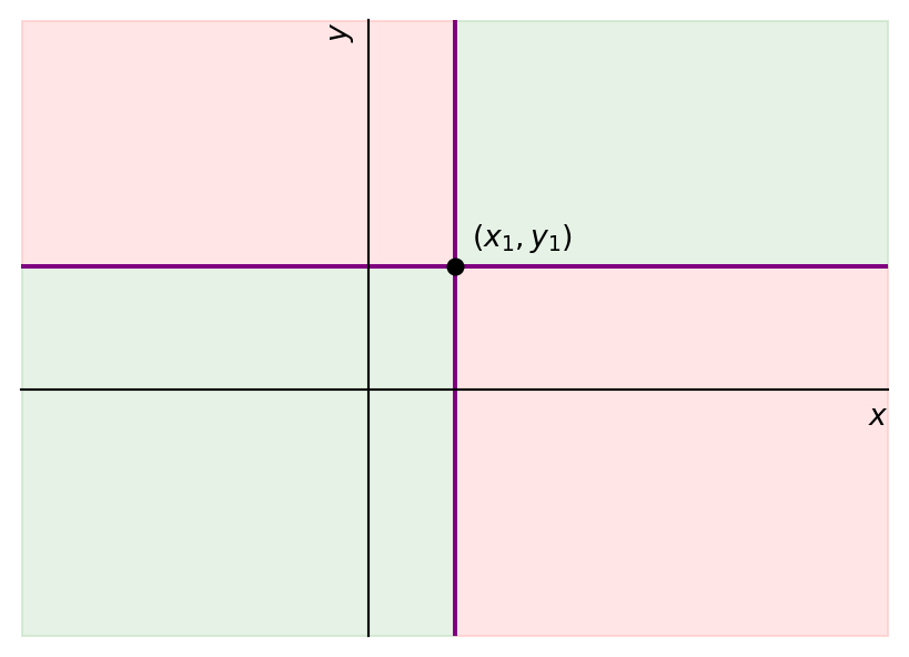
Remark 5.4. We can visualise the above nicely. We take the first $(x_1,y_1) \in \R^2$ as our base point if you will (but could equally well take the second one in that role, it’s all symmetric), and then we investigate where $(x_2,y_2) \in \R^2$ is located relative to this base point to decide whether we’re dealing with a concordant or discordant pair. Cf. Figure 5.1: all points in the green region satisfy Equation 5.4 i.e. make for a concordant pair of points with $(x_1,y_1)$, while all points in the red region satisfy Equation 5.5 i.e. make for a discordant pair of points with $(x_1,y_1)$.

Note that we do not classify the points on the purple lines i.e. those points $(x_2,y_2) \in \R^2$ with $x_2=x_1$ or $y_2=y_1$. That’s because it’s not clear which way we should go with those, and importantly we simply don’t need to worry about them! Here’s the reason why. Ultimately we’re interested in probabilities (we’ll pursue this further below). And given $(x_1,y_1) \in \R^2$, due to our assumption that $X$ and $Y$ are continuous random variables the probability that the second point ends up on one of the purple lines is \[\P(X=x_1 \text{ or } Y=y_1) \leq \P(X=x_1) + \P(Y=y_1)=0\] (recall Equation A.14) i.e. these points are irrelevant.

Figure 5.1: Visualising concordance and discordance relative to the base point $(x_1,y_1)$

Of course, the subtlety is that if we go through this process of generating two samples $(x_1,y_1)$ and $(x_2,y_2)$ from $(X,Y)$ and compare them, then generally (unless we have some trivial form of dependency) we won’t always get the same result. Rather, if we do this say $n$ times, then some proportion of those $n$ pairs of points will be concordant while the others are discordant. So what we’re interested in is, if we carry out this process once, the probability that we get a concordant pair of samples and the probability that we get a discordant pair of samples (these two are of course each others complement i.e. they add up to $1$, as argued in Remark 5.4) i.e. what proportion of outcomes results in concordance resp. discordance in the limit for $n \to \infty$³. And this is exactly what Kendall’s tau, denoted by $\tau$, does: \[\begin{align*} \tau &= \text{the prob that we get a \emph{concordant} pair of samples} \\ & \qquad - \text{the prob that we get a \emph{discordant} pair of samples.} \end{align*} \tag{5.6}\]

³ This is of course nothing but the Law of Large Numbers, cf. Section A.7 as well as yet another manifestation of the same ideas that were behind the Monte Carlo simulation technique from Chapter 1

To express $\tau$ in a proper grown up mathematical definition, observe that the process of generating two samples $(x_1,y_1)$ and $(x_2,y_2)$ from $(X,Y)$ can equivalently be expressed as: make two independent copies $(X_1,Y_1)$ and $(X_2,Y_2)$ of $(X,Y)$, and generate a sample $(x_1,y_1)$ resp. $(x_2,y_2)$ from $(X_1,Y_1)$ resp. $(X_2,Y_2)$. Using Equation 5.4 and Equation 5.5 we can then equivalently write Equation 5.6 as \[\begin{align*} \tau &= \P \big( (X_2-X_1)(Y_2-Y_1)>0 \big) \\ & \qquad - \P \big( (X_2-X_1)(Y_2-Y_1)<0 \big). \end{align*}\]

Definition 5.2 Let $(X,Y)$ be a pair of continuous random variables, and let $(X_1,Y_1)$ and $(X_2,Y_2)$ be independent copies of $(X,Y)$. Then Kendall’s tau is the measure of dependence (for $(X,Y)$) defined as \[\begin{align*} \tau &= \P \big( (X_2-X_1)(Y_2-Y_1)>0 \big) \\ & \qquad - \P \big( (X_2-X_1)(Y_2-Y_1)<0 \big) \in [-1,1]. \end{align*} \tag{5.7}\]

Some notes:

Note that the two probs in Equation 5.7 are each other’s complements i.e. \[\P \big( (X_2-X_1)(Y_2-Y_1)>0 \big)=1-\P \big( (X_2-X_1)(Y_2-Y_1)<0 \big), \tag{5.8}\] because \[\begin{align*} \P \big( (X_2-X_1)(Y_2-Y_1)=0 \big) &= \P \big( X_1=X_2 \text{ or } Y_1=Y_2 \big) \\ &\leq \P(X_1=X_2)+\P(Y_1=Y_2) \\ &= 0, \end{align*} \] the final equation by Lemma A.1 (note that this is essentially the same observation we already made in Remark 5.4 about the points on the purple lines in the visual there).

So Kendall’s tau could equally well have been defined using one of these two probs only, as the other is then known as well. It’s just that Equation 5.7 is convenient because it gives a nice symmetric range of possible values from $-1$ to $1$, with the sign having a meaning, so similar in that sense to the correlation coefficient from Section 5.2.
A value of $\tau$ close to $1$ (resp. $-1$) means that $\P \big( (X_2-X_1)(Y_2-Y_1)>0 \big)$ is close to $1$ (resp. $0$) and (hence) $\P \big( (X_2-X_1)(Y_2-Y_1)<0 \big)$ is close to $0$ (resp. $1$), that is: any two samples from $(X,Y)$ are very likely to be concordant (resp. discordant), or in the language used earlier in this section: $X$ and $Y$ are very likely to “move in the same direction” (resp. to “move in opposite directions”). Of course, $\tau=1$ (resp. $-1$) means that concordance (resp. discordance) happens with probability $1$.

Aside: why don’t you just say “happens for certain” in that last sentence above Kees? Well because that’s generally not entirely the same! For instance, a $\mathcal{N}(0,1)$ distributed random variable takes any value other than say $2.5$ with probability $1$ (recall Equation A.14), but that doesn’t mean it’s impossible for it to take the value $2.5$!
A value of $\tau$ close to $0$ means that concordance and discordance are more or less equally likely to occur i.e. that neither “$X$ and $Y$ tend to move in the same direction” nor “$X$ and $Y$ tend to move in opposite directions” are true really.

Nothing to get used to a new concept as working it out a simple enough example in which you can easily convince yourself whether or not it does the right thing! Here is one.

Example 5.2 Consider a pair $(X,Y)$ of continuous random variables where $Y=aX$ for some $a>0$. Then obviously if we create two independent copies $(X_1,Y_1)$ and $(X_2,Y_2)$ we also have $Y_1=aX_1$ and $Y_2=aX_2$ and we can work out \[\begin{align*} \P \big( (X_2-X_1)(Y_2-Y_1)>0 \big) &= \P \big( (X_2-X_1)(aX_2-aX_1)>0 \big) \\ &= \P \big( a(X_2-X_1)^2>0 \big) \\ &= \P \big( (X_2-X_1)^2>0 \big) \\ &= 1, \end{align*} \] where in the final step we used that it is obviously always true that $(X_2-X_1)^2 \geq 0$ and also \[\P \big( (X_2-X_1)^2=0 \big)=\P(X_1=X_2)=0\] (using Lemma A.1).

So to compute Kendall’s tau we first note that (cf. Equation 5.8) \[\P \big( (X_2-X_1)(Y_2-Y_1)<0 \big)=1-\P \big( (X_2-X_1)(Y_2-Y_1)>0 \big)=0\] and hence from Equation 5.7 \[\tau=1-0=1.\]

As mentioned in the second bullet point in Definition 5.2, this is the largest value that $\tau$ can have and it indicates that concordance happens with probability $1$ i.e. that $X$ and $Y$ “move in the same direction” with probability $1$. Well indeed, since $Y=aX$ and $a>0$, if $X$ grows then $Y$ is guaranteed to grow as well!

Can you guess what happens if we change $a>0$ to $a<0$?

Finally in this section, recall that in Remark 5.3 we discussed that the correlation coefficient is not truely a “measure of dependence” as it also depends on the marginal distributions of $X$ and $Y$. A true measure of dependence only needs to know what the dependency structure between $X$ and $Y$ is i.e. what its copula is and doesn’t care about the marginal distributions. The below result shows that this is true for Kendall’s tau, by even giving an explicit expression for $\tau$ in terms of the copula of $(X,Y)$ only!

Proposition 5.2 Let $(X,Y)$ be a jointly continuous pair of random variables (recall that this is slightly stronger than demanding that $X$ and $Y$ are each continuous random variables, cf. Remark A.2) with unique copula $C$ describing its dependency structure (recall from Theorem 3.1 that we know that this $C$ exists).

Suppose that $C$ is smooth enough for its mixed partial derivative \[C^{(1,1)}(u,v) := \frac{\partial^2 C(u,v)}{\partial u \partial v}=\frac{\partial^2 C(u,v)}{\partial v \partial u}\] (recall from an earlier course that these two derivatives are always the same) to exist on $(0,1)^2$. Then Kendalls tau $\tau$ from Definition 5.2 can be expressed in terms of $C$ as follows: \[\tau=4 \iint_{(0,1)^2} C(u,v) C^{(1,1)}(u,v) \d (u,v)-1. \tag{5.9}\]

Some notes:

Recall that the two-dimensional integral in Equation 5.9 can be worked out as a repeated one-dimensional integral and that the order in which you do that does not matter, i.e. you can equally well write it as a $\iint ... \d u \d v$ integral or as a $\iint ... \d v \d u$ integral, cf. Section A.3.2 if you’d like a quick reminder.
The assumptions we made here (on the smoothness of $C$ in particular) can be relaxed, however in the more general case the relationship Equation 5.9 needs to involve a generalisation of two-dimensional Riemann integrals and we don’t really want to go there in this course. If you’re interested, see McNeil, Frey, and Embrechts (2015) e.g.

Proof. Outline only, as we won’t have time to discuss this in the lectures sadly but I do want to give an impression for those of you interested. If you want full details, see e.g. McNeil, Frey, and Embrechts (2015).

Obviously we need to start with $\tau$ as defined in Definition 5.2 and then work our way towards Equation 5.9. So we need to somehow find a way to express probabilities for (independent copies of) $(X,Y)$ in terms of the copula $C$ of $(X,Y)$. In general, as we know well (you hadn’t forgotten about Equation 3.9 eh??), such probabilities will depend not only on the copula but also on the marginal distributions. It’s just that these specific probabilities we consider in Definition 5.2 turn out to depend on $C$ only.

The key idea is this: a probability for a pair is determined by its joint cdf (and/or joint pdf in case that one exists, which it does under our assumptions). Sklar’s theorem (Theorem 3.1) tells us how to link the joint cdf to the copula (plus the marginal distributions). So this gives a way to link probabilities/Kendall’s tau to the copula plus marginal distributions. The rest is “just” some elbow grease to do the algebra, and observing at some point along the way that it turns that the marginal distributions are actually irrelevant here.

A walkthrough for those of you who are interested: let $F_{X,Y}$ resp. $f_{X,Y}$ be the joint cdf resp. pdf (recall Section A.3.3) of $(X,Y)$, the same for the marginal cdf and pdf of $X$ and $Y$, and let $(X_1,Y_1)$ and $(X_2,Y_2)$ be independent copies of $(X,Y)$. Using Sklar’s theorem (Theorem 3.1) you can establish \[f_{X,Y}(x,y)=C^{(1,1)} \big( F_X(x),F_Y(y) \big) f_X(x) f_Y(y).\] Then observe that \[\begin{align*} \psi(x,y) &:= \P \big( X_2>X_1 \ \& \ Y_2>Y_1 \, \big| \, (X_2,Y_2)=(x,y) \big) \\ &= \P(x>X_1 \ \& \ y>Y_1) \\ &= \P(X_1 \leq x \ \& \ Y_1 \leq y) \\ &=F_{X,Y}(x,y) \\ &=C \big( F_X(x),F_Y(y) \big) \end{align*} \] (the third equation using Equation A.14 and the final one Sklar’s theorem) so that the Law of Total Expectation (cf. Section A.4) yields \[\P(X_2>X_1 \ \& \ Y_2>Y_1)=\E[\psi(X_2,Y_2)],\] the right hand side of which is by def (cf. Equation A.40) \[\iint_{\R^2} \psi(x,y) f_{X,Y}(x,y) \d (x,y).\] This can be worked out, using the above expressions for $\psi$ and $f_{X,Y}$, to \[\iint_{(0,1)^2} C(u,v) C^{(1,1)}(u,v) \d (u,v).\] You can express $\P(X_2<X_1 \ \& \ Y_2<Y_1)$ in the same way (or be smart and realise that it must be the same as $\P(X_2>X_1 \ \& \ Y_2>Y_1)$), and then you have everything you need to work out Equation 5.7 and to arrive at Equation 5.9.

One more quick example then!

Example 5.3 Consider a jointly continuous pair $(X,Y)$ where $X$ and $Y$ are independent. We could compute Kendall’s tau for such a pair via the def Definition 5.2, but recall that we also quite well know what the copula of this pair is, indeed nothing but the independence copula $C(u,v)=uv$ from e.g. Example 3.3, and so we could also use Proposition 5.2!

Note that \[\begin{align*} C^{(1,1)}(u,v) &= \frac{\partial^2}{\partial u \partial v} uv \\ &= \frac{\partial}{\partial u} \left( \frac{\partial}{\partial v} uv \right) \\ &= \frac{\partial}{\partial u} u \\ &= 1 \end{align*} \] and so we get from Proposition 5.2 that \[\begin{align*} \tau &= 4 \iint_{(0,1)^2} C(u,v) C^{(1,1)}(u,v) \d (u,v)-1 \\ &= 4 \iint_{(0,1)^2} uv \d (u,v)-1 \\ &= 4 \int_0^1 \left( \int_0^1 uv \d u \right) \d v -1 \\ &= 4 \int_0^1 \left( \left. \frac{u^2}{2} v \right|_{u=0}^{u=1} \right) \d v -1 \\ &= 4 \int_0^1 \frac{v}{2} \d v -1 \\ &= 4 \cdot \frac{1}{4}-1 \\ &= 0, \end{align*} \] reassuringly the same value as in Exercise 5.2! :).

5.4 Tail dependence

One more then: tail dependence! This one focusses on what you might call “extreme events”: if in a pair $(X,Y)$ one of the two takes a very large (or very small) value, does that make it more likely that the other wil take a very large (or very small) value as well?

A nice example where such questions play an important role is in insurance. Imagine that you are working for an insurance company and have sold home insurances (i.e. insurance policies that reimburse home owners in the case of damage to their house) for quite a few homes in the lovely Peak District⁴. Let $X$ and $Y$ represent the damage amount claimed (during a year say) for House 1 and House 2 say. If these two houses are in quite different parts of the Peak District, then you’ll agree that serious damage to the one house likely has no particular predicting effect on any damage to the other house. However, if they are located in the same village then you need to account for instance for the following effect: if a large flood occurs that damages one of the houses, then it is quite likely that the other house gets damaged as well. That is to say, a large claim for House 1 (i.e. value for $X$) is quite likely to come with a large claim for House 2 (i.e. value for $Y$ as well)!

⁴ That beautiful quite hilly area just to the east of Manchester — if you’ve never been there you should def go have a look!

And here is the potentially ugly financial bottomline: (non-life) insurance companies operate on the principle that relatively small amounts of premiums (=cost to buy an insurance product) paid in by many is used to reimburse some only (only those that are unlucky enough to suffer from a relatively rare event with serious consequences). If these insurance policies can reasonably be assumed to behave independently (at least when it comes to the occurence of large claims) and you sell enough of them, then you can pretty accurately predict how much you’ll have to pay in claims every year (there is a claim every now and then, at a relatively predictable frequency) and set your premiums to a level sufficient to cover these (plus cost of running the business etc.). However in a “large claim tends to come with another large claim” situation as in the example in the previous paragraph, (large) claims are much more likely to come in waves of quite a few at (more or less) the same time, and if you’re not adequately financially prepared for that then such a wave could easily more than wipe out all the company’s reserves, sending it into bankruptcy, leaving the claimants out of pocket, and you having to tell your kids that the summer hols will be a week in a leaky and moldy hotel room in Blackpool rather than a month in a fancy resort somewhere warm and sunny! So you better get a proper grip of this, i.e. get your tail dependence modelling right (enough)!

5.4.1 Dealing with the influence of marginal distributions

In principle formulating the concept of tail dependence in terms of maths is not very difficult. There is just one somewhat complicating factor we need to discuss first: we mentioned that we are interested in the “very large” (or “very small”) values of the random variables we are considering, but what does that exactly mean? Indeed, after a moment of thought you’ll agree that this very much depends on the distribution of that random variable. For instance, if $X \sim \mathcal{N}(0,1)$ then $X$ has range⁵ $\R$, and a “very large” value would naturally be some very large element of $\R$ (maybe $100$ or $1000$ or …) resp. “very small” some very negative element of $\R$ (maybe $-100$ or $-1000$ or …), while if say $X \sim \text{Unif}(a,b)$ then $X$ has range $(a,b)$, and a “very large” value would naturally be some number close to but less than $b$ (maybe $b-0.001$ e.g.) resp. “very small” some number close to $a$ but larger than (maybe $a+0.001$ e.g.).

⁵ Don’t forget about the discussion around Equation A.18!

So we need a way to specify what “very large” values resp. “very small” values of a random variable, say $Z$ for now, exactly are while properly accounting for the influence of its range and distribution. The good news is that actually you already know a good way to do this, at least for the special case that $Z \sim \mathcal{N}(0,1)$! Let’s recall that one briefly, and then use the same ideas to deal with any distribution/range for $Z$.

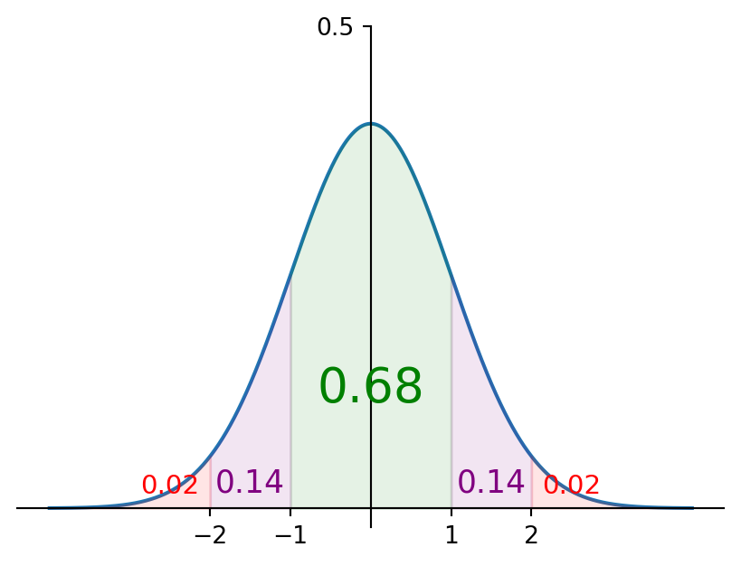
Example 5.4 Recall the picture associated with $Z \sim \mathcal{N}(0,1)$ you know so very well, already from before uni I would assume for most/all of you: the pdf $f_Z$ of this $Z$ (the famous “Bell curve”, recall its expression from Appendix B) with some associated values for the area under that graph (rounded to two decimals), cf. Figure 5.2. Of course, the area under a part of that graph gives a probability, for instance (taking the rounded areas in the graph as exact): $\P(Z \in [-1,1])=0.68$, $\P(Z>0)=\P(Z \geq 0)=0.68/2+0.14+0.02=0.5$ etc. (recall Equation A.14 if the switch from “$>0$” to “$\geq 0$” bugs you), you know this stuff all too well.

But here’s another thing we can read from this graph: the probability that $Z$ takes a value smaller than $-2$ is (only) $0.02$. So $-2$ is a pretty small value for $Z$ to take no? Similarly, the probability that $Z$ takes a value larger than $2$ is (only) $0.02$, making $2$ a pretty large value for $Z$ right?

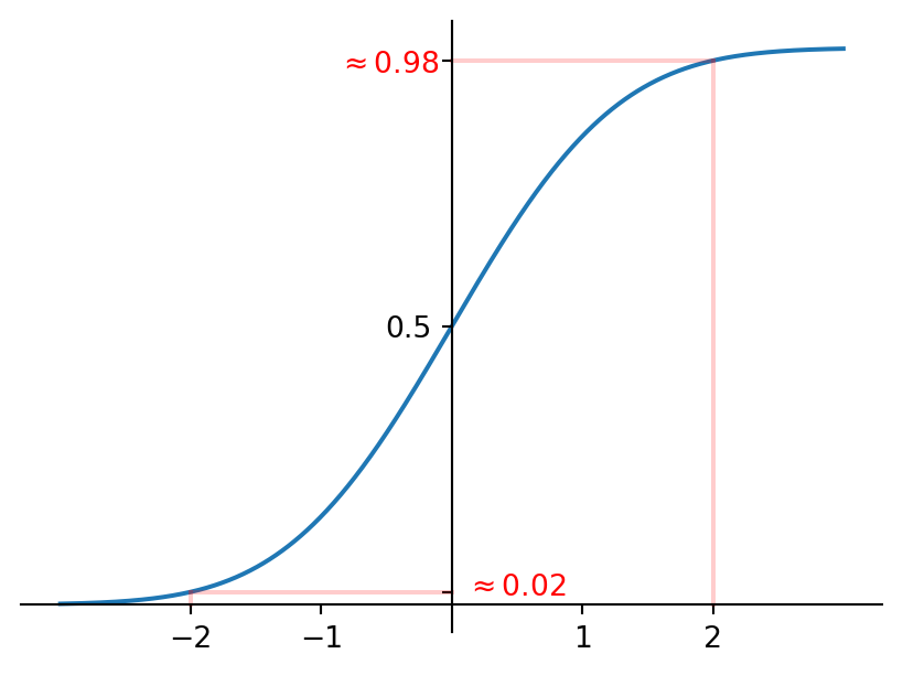
Figure 5.2: The pdf $f_Z$ of a $\mathcal{N}(0,1)$ distribution with associated areas (rounded to two decimals) under the graph

Note that we can of course equally well see this from the cdf $F_Z$ of $Z$. After all for any $x \in \R$, $F_Z(x)$ is by def (cf. Section A.1.1) equal to $\P(Z \leq x)$ or, visually, to the area under the graph of $f_Z$ where you walk on the horizontal axis from $-\infty$ up until $x$. In particular: \[\P(Z \leq -2)=F_Z(-2) \approx 0.02\] and \[\P(Z > 2)=1-\P(Z \leq 2)=1-F_Z(2) \approx 0.02.\] See also Figure 5.3.

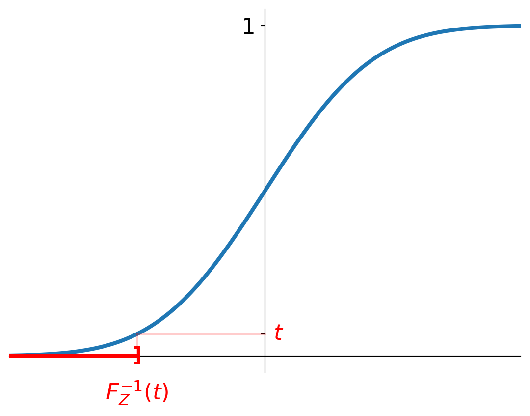
Figure 5.3: The cdf $F_Z$ of a $\mathcal{N}(0,1)$ distribution

In fact, we could also invert this argument: a sensible way to specify what the “very small” values of $Z$ are is to choose a $t \in (0,1)$ close to $0$ and to solve $x \in \R$ from the equation $F_Z(x)=t$ i.e. $x=F_Z^{-1}(t)$ (we can safely use the classic inverse here, recall the discussion in Section 2.2.1). This $x$ then gives an upper bound for what we consider the “very small” values: it holds that \[\begin{align*} \P(Z \leq x) &= \P \big( Z \leq F_Z^{-1}(t) \big) \\ &= F_Z \big( F_Z^{-1}(t) \big) \\ &= t \end{align*} \tag{5.10}\] (where the final equality holds because we’re using the classic inverse here — or, if you prefer, since $F_Z$ is continuous this also follows from Lemma 2.1 ii) i.e. in words: the probability that $Z$ takes a value in the interval \[(-\infty,x]= \big( -\infty,F_Z^{-1}(t) \big] \tag{5.11}\] is (only) $t$ (recall: close to $0$). For example, if we take $t=0.02$ then we get the interval \[\big( -\infty,F_Z^{-1}(0.02) \big] \approx (-\infty,-2].\] So if were to produce 100 samples from $Z$, then we should expect only 2 of these to end up in that interval i.e. to be less than or equal to $-2$. Obviously, the closer we move $t$ to $0$, the more the interval Equation 5.11 moves to the left on the horizontal axis. See also Figure 5.4 (a).

Turning our attention to the “very large” values of $Z$, we can specify these in the same way, just at the other extreme if you will: take a $t \in (0,1)$ close to $1$ and again solve $x \in \R$ from the equation $F_Z(x)=t$ i.e. $x=F_Z^{-1}(t)$. This $x$ is then a lower bound for what we consider the “very large” values: \[\begin{align*} \P(Z > x) &= \P \big( Z > F_Z^{-1}(t) \big) \\ &= 1-\P \big( Z \leq F_Z^{-1}(t) \big) \\ &= 1-F_Z \big( F_Z^{-1}(t) \big) \\ &= 1-t, \end{align*} \tag{5.12}\] which is close to $0$ since we took $t$ close to $1$. Indeed, this tells us that the probability that $Z$ takes a value in the interval \[(x,\infty)=\big( F_Z^{-1}(t), \infty)\] is (only) $1-t$. The fact that we used an open interval here and a closed one in Equation 5.11 is arbitrary and makes no actual difference anyway (recall Equation A.14). See Figure 5.4 (b). For example, if we take $t=0.999$ then this interval becomes \[\big( F_Z^{-1}(0.999), \infty) \approx (3.09,\infty)\] i.e. if we produce 1000 samples from $Z$, then we should expect that only one of these is larger than $3.09$ (if you’re not sure: our choice of $t=0.999$ ensures that with probability $0.999$, such a sample is less than or equal to $3.09$!).

Of course, this whole discussion leaves us with the frustration that it does not yet tell us which values for $t$ we should exactly choose — we’ll address that in Section 5.4.2!

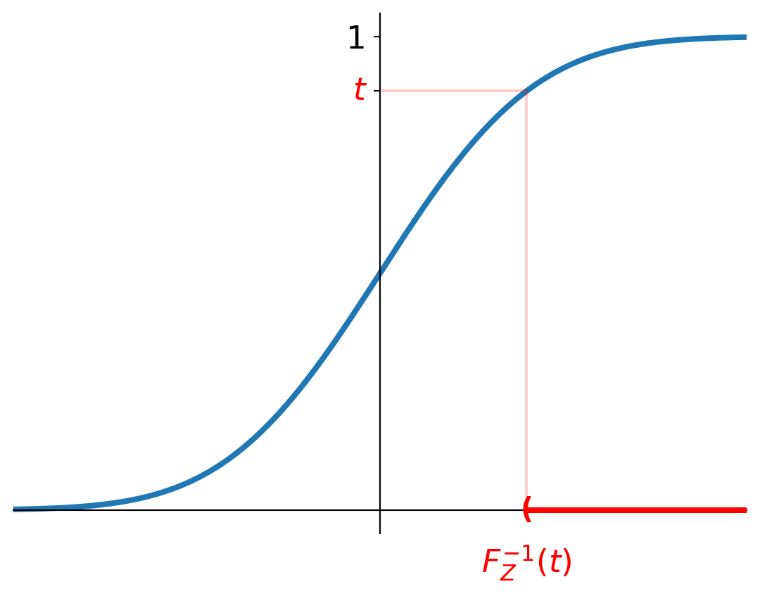
(a) “Very small”: the interval $(-\infty,F_Z^{-1}(t)]$, visualised in red, for $t$ close to $0$. Note that as we let $t$ decrease towards $0$, the upper bound of this interval i.e. $F_Z^{-1}(t)$ moves towards $-\infty$

The beauty of the thinking via the (inverse) cdf in the above example is that we can use it in exactly the same way to naturally specify what “very large” and “very small” values are for a random variable $Z$ with any distribution/range! Indeed:

Lemma 5.1 Let $Z$ be a random variable with continuous cdf $F_Z$ and inverse cdf $F_Z^{-1}$ (which may have to be the generalised inverse as introduced in Section 2.2.1). Then:

For $t$ close to $0$, the interval \[\big( -\infty,F_Z^{-1}(t) \big]\] contains the “very small” values that $Z$ can take. The justification is that the probability that $Z$ ends up in this interval, i.e. $\P \big( Z \leq F_Z^{-1}(t) \big)$, equals $t$ (cf. Equation 5.10).
For $t$ close to $1$, the interval \[\big( F_Z^{-1}(t), \infty)\] contains the “very large” values that $Z$ can take. The justification is that the probability that $Z$ ends up in this interval, i.e. $\P \big( Z > F_Z^{-1}(t) \big)$, equals $1-t$ (cf. Equation 5.12).

When used in this context, the inverse cdf $F_Z^{-1}$ is often called the quantile function.

5.4.2 Formulating the tail dependence parameters

Back to our main goal now, which at the start of Section 5.4 we wrote to be: if in a pair $(X,Y)$ one of the two takes a very large (or very small) value, does that make it more likely that the other wil take a very large (or very small) value as well? Without loss of generality we can let $X$ be the one that we know to take a very large (resp. very small) value, and then wonder whether this makes the probability that $Y$ also takes a very large (resp. very small) value larger than it is without this knowledge.

Focussing on “very large” first, this translates to the question whether the conditional probability \[\P(Y \text{ takes a very large value} \, | \, X \text{ takes a very large value})\] is larger than the (marginal) probability \[\P(Y \text{ takes a very large value}).\] Making this more precise using Lemma 5.1, this translates further to: for $t$ close to $1$, is the conditional probability \[\P \big( Y>F_Y^{-1}(t) \, \big| \, X>F_X^{-1}(t) \big)\] larger than the (marginal) probability \[\P \big( Y>F_Y^{-1}(t) \big).\]

The final piece of the puzzle is now the following. Both these probabilities depend on $t$, so how do we actually make that comparison exactly? I mean, it could well be that for some $t$ one might be larger while for other $t$ the other is larger no? We make the following choice here: as we are interested in the “most extreme” values, we would like to compare them for $t$ as close to $1$ as possible. We can’t set $t$ equal to $1$ sadly⁶, so the next best thing is then to compare their limits as $t \uparrow 1$ (provided they exist), so that our question becomes: is the conditional probability \[\lim_{t \uparrow 1} \P \big( Y>F_Y^{-1}(t) \, \big| \, X>F_X^{-1}(t) \big) \tag{5.13}\] larger than the (marginal) probability \[\lim_{t \uparrow 1} \P \big( Y>F_Y^{-1}(t) \big).\] The last bit of manipulation: since $\P \big( Y>F_Y^{-1}(t) \big)=1-t$ (the same computation as in Equation 5.12) this second limit is just $0$ (no matter what distribution $Y$ has!) and so the really final formulation of our question is: is the conditional probability Equation 5.13 larger than $0$?

⁶ Because then the events $\{ X>F_X^{-1}(t) \}$ and $\{ Y>F_Y^{-1}(t) \}$ are both empty, as we’re then asking for the impossible namely for $X$ resp. $Y$ to take a value larger than their respective largest possible values!

Making the switch to “very small”, that all works in the same way: we’re then wondering whether the conditional probability \[\P(Y \text{ takes a very small value} \, | \, X \text{ takes a very small value})\] is larger than the (marginal) probability \[\P(Y \text{ takes a small large value}),\] which we can again translate using Lemma 5.1 and then take the limit for $t \downarrow 0$ to see that this is the same question as whether the conditional probability \[\lim_{t \downarrow 0} \P \big( Y \leq F_Y^{-1}(t) \, \big| \, X \leq F_X^{-1}(t) \big)\] is larger than $0$.

All of this brings us now to the following conclusion:

Definition 5.3 Let $(X,Y)$ be a pair of random variables with continuous marginal cdf’s $F_X$ and $F_Y$. Then the upper tail dependence parameter is defined as the limit (provided it exists) \[\lambda_U = \lim_{t \uparrow 1} \P \big( Y>F_Y^{-1}(t) \, \big| \, X>F_X^{-1}(t) \big) \in [0,1]\] and the lower tail dependence parameter as the limit (provided it exists) \[\lambda_L = \lim_{t \downarrow 0} \P \big( Y \leq F_Y^{-1}(t) \, \big| \, X \leq F_X^{-1}(t) \big) \in [0,1].\]

We can interpret the value of $\lambda_U$ as follows (direct consequence of the discussion we had above this def!):

If $\lambda_U=0$ then $X$ taking a very large value does not make the probability that $Y$ also takes a very large value any larger.
If $\lambda_U \in (0,1)$ then $X$ taking a very large value does increase the probability that $Y$ also takes a very large value. The larger $\lambda_U$, the more increased this probability for $Y$ is.
If $\lambda_U=1$ then $X$ taking a very large value implies (with probability $1$) that $Y$ also takes a very large value.

For $\lambda_L$ the interpretation is analogue, just replace every “very large value” above by “very small value”.

Example time!

Example 5.5 Consider one of our favourite simple examples: a pair $(X,Y)$ with continous marginal cdf’s $F_X$ and $F_Y$, where $X$ and $Y$ are independent. Looking at the interpretations in Definition 5.3, since $X$ does not influence $Y$ in any way, we would expect that in this case we have $\lambda_U=\lambda_L=0$. Let’s check!

For any $t \in (0,1)$ we can relatively easily work out \[\begin{align*} \P \big( Y>F_Y^{-1}(t) \, \big| \, X>F_X^{-1}(t) \big) &= \frac{\P \big( Y>F_Y^{-1}(t) \, \& \, X>F_X^{-1}(t) \big)}{\P \big( X>F_X^{-1}(t) \big)} \\ &= \frac{\P \big( Y>F_Y^{-1}(t) \big) \P \big( X>F_X^{-1}(t) \big)}{\P \big( X>F_X^{-1}(t) \big)} \\ &= \P \big( Y>F_Y^{-1}(t) \big) \\ &= 1-t, \end{align*} \] where the first equation uses the def of conditional probabilities (cf. Equation A.42), the second the independence (cf. Equation A.53), and the final one uses the same computation as in Equation 5.12. So indeed we get from Definition 5.3 that \[\begin{align*} \lambda_U &= \lim_{t \uparrow 1} \P \big( Y>F_Y^{-1}(t) \, \big| \, X>F_X^{-1}(t) \big) \\ &= \lim_{t \uparrow 1} 1-t \\ &= 0. \end{align*} \]

You can do the analogue computation for $\lambda_L$ by yourself.

We conclude this section and chapter with the following. Recall that in Section 5.3 we saw that Kendall’s tau is a true (as opposed to the correlation coefficient) “measure of dependence” in the sense that it only depends on the copula of a pair $(X,Y)$ and not on the marginal distributions of $X$ and $Y$. We showed this quite explicitly, by expressing Kendall’s tau in terms of that copula (cf. Proposition 5.2). It turns out that also the tail dependence parameters $\lambda_U$ and $\lambda_L$ are true “measures of dependence”⁷, and again we can show this by deriving an explicit expression for them in terms of the copula:

⁷ Here we get some extra reward for the careful thinking we did in Section 5.4.1 about how we should define “large values” and “small values” for $X$ and $Y$, and that we did that in such a way that we eliminated the influence of the marginal distributions of $X$ and $Y$ from the expressions for $\lambda_U$ and $\lambda_L$ (even though that may not be immediately apparent from these expressions)!

Proposition 5.3 Let $(X,Y)$ be a pair of random variables with continuous marginal cdf’s $F_X$ and $F_Y$, with (unique) copula $C$ (recall Sklar’s theorem Theorem 3.1) and with upper and lower tail dependence parameter as defined in Definition 5.3. Then we have that \[\lambda_U=2-\lim_{t \uparrow 1} \frac{1-C(t,t)}{1-t} \tag{5.14}\] and \[\lambda_L=\lim_{t \downarrow 0} \frac{C(t,t)}{t}. \tag{5.15}\]

A note:

typically it is the case that \[\lim_{t \uparrow 1} C(t,t)=C(1,1)=1\] and \[\lim_{t \downarrow 0} C(t,t)=C(0,0)=0\] (recall from Remark 3.1 that any copula has the property that $C(1,1)=1$ and $C(0,0)=0$), which means that in both Equation 5.14 and Equation 5.15, the numerator and denominator in the limit both tend to $0$. Recall that for evaluating such limits, l’Hôpital’s rule can be damn handy!

Proof. The proof follows the same line of thinking that we also used in the proof of Proposition 5.2: $\lambda_U$ and $\lambda_L$ are both defined in terms of probabilities for the pair $(X,Y)$. Any such probability can (in principle) be expressed using the joint cdf $F_{X,Y}$, and Sklar’s theorem Theorem 3.1 tells us how the joint cdf can be expressed in terms of the copula $C$ and the marginal cdf’s $F_X$ and $F_Y$. And then, after we have made these substitutions, we hope that these marginal cdf’s somehow cancel out and we’re left with an expression in terms of the copula only!

This works out very quickly for $\lambda_L$. Indeed for any $t \in (0,1)$ we get that \[\begin{align*} \P \big( Y \leq F_Y^{-1}(t) \, \big| \, X \leq F_X^{-1}(t) \big) &= \frac{\P \big( Y \leq F_Y^{-1}(t) \, \& \, X \leq F_X^{-1}(t) \big)}{\P \big( X \leq F_X^{-1}(t) \big)} \\ &= \frac{F_{X,Y} \big( F_X^{-1}(t),F_Y^{-1}(t) \big)}{t} \\ &= \frac{C(t,t)}{t}, \end{align*} \] and now just take the limit for $t \downarrow 0$ on both sides. Note that above:

the first equation uses the def of conditional probabilities (cf. Equation A.42);
for the second, recall that by very def, \[F_{X,Y}(x,y)=\P(X \leq x \ \& \ Y \leq y) \quad \text{for all } x,y \in \R\] (cf. Section A.3.1) which we used in the numerator with the choices $x=F_X^{-1}(t)$ and $y=F_Y^{-1}(t)$, while in the denominator we used the same computation as in Equation 5.10;
and for the third equation we used Proposition 3.1 with the choices $u=t$ and $v=t$.

The proof for $\lambda_U$ works in exactly the same way, just the algebra is a bit more fiddly because the probabilities there are a bit less “cdf friendly” and need to be massaged a bit more.

Example 5.6 Let’s pick up the situation from Example 5.5 again. We had already computed that $\lambda_U=0$ there, working from the definition Definition 5.3. However, we also know quite well by now what the copula is that describes the dependency structure in this pair, indeed the independence copula which we have encountered several times before: \[C(u,v)=uv \quad \text{for all } u,v \in (0,1). \tag{5.16}\] If we work out $\lambda_U$ again, now using Proposition 5.3, we reassuringly get the same result: \[\begin{align*} \lambda_U &= 2-\lim_{t \uparrow 1} \frac{1-C(t,t)}{1-t} \\ &= 2-\lim_{t \uparrow 1} \frac{1-t^2}{1-t} \\ &= 2-\lim_{t \uparrow 1} \frac{(1-t)(1+t)}{1-t} \\ &= 2-\lim_{t \uparrow 1} 1+t \\ &= 2-2=0. \end{align*} \] Note that as we manipulate this limit, we do this with the understanding that $t \in (0,1)$, in particular $t<1$. So we get that $C(t,t)=t^2$ immediately from Equation 5.16 without needing to worry that Equation 5.16 does not cover the case $t=1$. Further, this limit is simple enough that an easy factorisation gets rid of the $0/0$ issue, but, as also mentioned in Proposition 5.3, l’Hôpital’s rule is a more general tool to attack such guys and could (of course) have been used here as well!

Remark 5.5. Some of you may be annoyed that we had to make this step to take the limit for $t \uparrow 1$ resp. $t \downarrow 0$ to come to Definition 5.3, as that obscures our intuitive understanding of what is happening somewhat. Let’s clarify a bit for those of you who are so invested (love you! ;)) — but don’t worry about this for assessment purposes.

Pick back up the exploration from above Definition 5.3, and define the functions $f,g: (0,1) \to [0,1]$ given by \[f(t)=\P \big( Y>F_Y^{-1}(t) \, \big| \, X>F_X^{-1}(t) \big) \quad \text{for } t \in (0,1)\] and \[g(t)=\P \big( Y>F_Y^{-1}(t) \big) \quad \text{for } t \in (0,1).\] Then, as defined in Definition 5.3, \[\lambda_U=\lim_{t \uparrow 1} f(t)\] (let’s assume it exists) and we argued above Definition 5.3 already that \[\lim_{t \uparrow 1} g(t)=0.\]

Now consider the situation that $\lambda_U >0$. Fix any $h \in (0,\lambda_U)$. Then, by def of these limits above, there exists a $t_0 \in (0,1)$ (dependent on $h$) so that $f(t)>g(t)+h$ for all $t \in (t_0,1)$. That is the following. There exists a cut-off point in the range of $X$ namely $F_X^{-1}(t_0) \in \R$ and a cut-off point in the range of $Y$ namely $F_Y^{-1}(t_0) \in \R$ so that if we consider a “very large” value of $X$ (resp. $Y$) any value larger than $F_X^{-1}(t_0)$ (resp. larger than $F_Y^{-1}(t_0)$), then the probability that $Y$ takes a very large value given that $X$ takes a very large value is at least $h$ larger than the (marginal) probability that $Y$ takes a very large value.

This provides a more detailed and precise (than given in Definition 5.3) understanding of what the value of $\lambda_U$ really means, but then again try to explain this level of subtlety to your manager with his cute Management degree at your fancy company… ;).

5.5 Some exercises

About the exercises

Each exercise has a (rough) indication of its difficulty, as follows:

*	easier: can be solved by (almost) only using relevant definitions/results,
**	medium: in addition to relevant definitions/results, needs a limited amount of work/creativity,
*******	harder: in addition to relevant definitions/results, needs a larger amount of work/serious creativity,
💀	warning: might make your brain hurt! These are mainly intended to provide some extra challenge for those of you keen on that and are generally quite hard. You don't need to worry about these too much for exam purposes.

The exam consists of mostly ** and *** level questions, some *, and possibly at most a few marks worth of 💀.

A bit of preaching: it is an incredibly important part of the study process to try and work on the exercises as much as possible. To become a better mathematician/learn new maths (and also to get a good exam mark ;)), above all you need to do it. And yes, of course that includes falling over things, and making mistakes, and getting stuck, and getting frustrated — all part of the game and what you’re supposed to be doing! Your lecturers have done that as well and still do it. What matters is that you don’t let that discourage you and that you make good use of the help and resources available to help you develop your skills. As part of that, many exercises have a hint in a block like this:

Hint (click to view)

Hint!

These are trying to help you on your way if you don’t know where to start or to provide some ideas if you get stuck. In spirit of the above, always have a look at these first and try again before you look at the full solution. (These hints are an extra service that won’t be available in the exam I’m afraid ;).)

Of course, we have our classes and there’s office hours, email etc. as well — I’m at any time very happy to help you with any questions you may have, and you should please never feel that any question is “too dumb” to ask!

Full/detailed solutions for the exercises will become available, just immediately below the exercises, immediately after our tutorial hour (you may have to refresh the page).

Warning

The exercises are some serious stuff this week I think: many not very easy and overall it’s quite a lot of work. That comes a bit with the territory of this chapter I’m afraid — the maths is not very easy and I do want to give you enough opportunity to work with the concepts. However please don’t let that discourage you too much: the upcoming chapters will be a bit lighter again, and of course in the exam I’ll take good care to carefully balance things.

Exercise 5.1 [**] Let $(X,Y)$ be a continuous pair of random variables with the followng properties:

$X$ is symmetrically distributed around $0$ in the sense that its pdf satisfies $f_X(-x)=f_X(x)$ for all $x \in \R$,
the first four moments of $X$ i.e. $\E[X], ..., \E[X^4]$ are all well defined and finite,
and $Y=X^2$.

Show that $\E[X]=\E[X^3]=0$.

Hint: write down the usual integral expression for these two expectations (cf. Equation A.16 and/or Equation A.17) and make use of the symmetry property of the pdf.
Deduce that $\rho(X,Y)=0$.
Denote by $F_X$ and $F_Y$ the (marginal) cdf’s of $X$ and $Y$. Using the same strategy as in part i, show that \[F_X(x)=1-F_X(-x) \quad \text{for all } x \in \R\] and use this relationship together with $Y=X^2$ to show that \[F_Y(x)=\begin{cases} 0 & \text{if } x<0 \\ 2 F_X(\sqrt{x})-1 & \text{if } x \geq 0 \end{cases} \] (note: the symmetry in the distribution of $X$ implies that $F_X(0)=1/2$, so despite the case distinction $F_Y$ is continuous — as it should be since $Y$ is a continuous random variable!).

It can be shown that the copula $C$ of $(X,Y)$ is given by the following impressively ugly contraption: \[C(u,v)=\max \left\{ \min \left\{ u, \frac{1+v}{2} \right\}-\frac{1-v}{2}, 0 \right\} \quad \text{for all } u,v \in (0,1). \tag{5.17}\]

[💀] Prove Equation 5.17. Lengthy and bit nasty algebra ahead young warrior!
Recall that in Exercise 3.4 we discussed pairs $(X,Y)$ where $Y=f(X)$. In that exercise we encountered the countermonotonicity and comonotonicity copulas. Why do we have a different copula in this case, i.e. not one of these two?
Compute the lower and upper tail dependence parameters, using Equation 5.17 and Proposition 5.3.

Hint: first show that for $t \in (0,1)$ the contraption Equation 5.17 simplifies to \[C(t,t)=\max \left\{ \frac{3t-1}{2},0 \right\}.\] Next show that for $t>0$ but close to $0$ we have $C(t,t)=0$, while for $t<1$ but close to $1$ we have $C(t,t)=(3t-1)/2$.
Can you give an explanation/interpretation for the values we found in parts vi?

There are a zillion concrete examples of pairs $(X,Y)$ as discussed in this question. We could for instance take $X \sim \text{Unif}(-a,a)$ for any $a>0$, or $X \sim \mathcal{N}(0,\sigma^2)$ for any $\sigma^2>0$.

One interesting point to note is the following. We saw in part ii that the correlation coefficient is $0$, and in part vi that the lower tail dependence parameter is also $0$. On the other hand, if $X$ and $Y$ are independent (so (very) different dependency structure/copula than we had in this question) we also have a correlation coefficient of $0$ (as you know well/can easily check) and lower tail dependence parameter of $0$ (cf. Example 5.5).

This observation hammers home the important point made in Section 5.1 already, namely that these measures of dependence are all necessarily “many-to-one”: there are many different dependency structures/copulas that share the same value for the correlation coefficient (or Kendall’s tau, or a tail dependence parameter)!

Hint (click to view)

For part i, use Equation A.17 and split the integral in two parts to write for $k \in \{1,3\}$ \[\begin{align*} \E[X^k] &= \int_{-\infty}^\infty x^k f_X(x) \d x \\ &= \int_{-\infty}^0 x^k f_X(x) \d x + \int_0^\infty x^k f_X(x) \d x, \end{align*} \] and then use e.g. a nice substitution to show that one integral is equal to $-1$ times the other!

For part ii, working from the def (cf. Definition 5.1) and using part i, a one liner!

For part iii, for the (marginal) cdf of $X$, use Equation A.12 to write \[F_X(x) = \P(X \leq x) = \int_{-\infty}^x f_X(y) \d y.\] Now think of a nice substitution which shows that that integral is also equal to $\P(X>-x)$!

For the (marginal) cdf of $Y$, start with $F_Y(x) = \P(Y \leq x)= \P(X^2 \leq x)$. Then consider the cases $x<0$ and $x \geq 0$ separately, and with a bit of algebra you get there.

For part iv, start by convincing yourself that using Sklar’s theorem (cf. Theorem 3.1) it is sufficient to show that \[F_{X,Y}(x,y)=C \big( F_X(x),F_Y(y) \big) \quad \text{for all } x,y \in \R. \tag{5.18}\] This route is possible because we already have an expression for $C$, and it avoids the inverse cdf’s needed in Proposition 3.1. Next work out the joint cdf, using the relationship between $X$ and $Y$. You should find that \[F_{X,Y}(x,y) = \begin{cases} 0 & \text{if } y<0 \text{ or } x \leq -\sqrt{y} \\ F_X(\sqrt{y})-F_X(x) & \text{if } y \geq 0 \text{ and } x \in (-\sqrt{y},\sqrt{y}] \\ F_X(\sqrt{y})-F_X(-\sqrt{y})=2 F_X(\sqrt{y})-1 & \text{if } y \geq 0 \text{ and } x > \sqrt{y}. \end{cases} \] Now go through the different cases in this expression one by one. In each case, work out the right hand side of Equation 5.18 (making optimal use of part iii) and deduce that Equation 5.18 indeed holds.

For part v, what is fundamentally different between the functions $f$ appearing in Exercise 3.4 and the one we have here??

For part vi, if you’re not sure about the second part of the hint, consider the function $f(t)=(3t-1)/2$ for $t \in [0,1]$. Note that it is continuous, and what is $f(0)$ resp. $f(1)$?

For part vii, recall that we discussed the interpretation in Definition 5.3. For the lower one the interpretation discussed there applies quite clearly, but for the upper one it is quite a bit more subtle! Indeed if you go by the textual interpretation given in Definition 5.3 only, you would rather expect to find $\lambda_U=1$ rather than $\lambda_U=1/2$. To explain this value, a closer look at the mathematical definition of $\lambda_U$ in Definition 5.3 is needed!

Full solution (click to view)

For part i, let’s do both in one argument (of course you can also do them separately if you prefer): for any $k \{1,3\}$ we get from Equation A.17 that \[\E[X^k] = \int_{-\infty}^\infty x^k f_X(x) \d x.\] The trick is to write this as the sum of two integrals: \[\E[X^k] = \int_{-\infty}^0 x^k f_X(x) \d x + \int_0^\infty x^k f_X(x) \d x,\] and to make the substitution $z=-x$ in the second (or first, if you prefer) integral to rewrite that one as \[\begin{align*} \int_0^\infty x^k f_X(x) \d x &= \int_{-\infty}^0 (-z)^k f_X(-z) \d z \\ &= -\int_{-\infty}^0 z^k f_X(z) \d z, \end{align*} \] where in the first equality a factor $-1$ vanishes by swapping the integral bounds, and the second uses that since $k$ is odd, $(-z)^k=-z^k$ as well as the symmetry of $f_X$. Hence \[\E[X^k] = \int_{-\infty}^0 x^k f_X(x) \d x -\int_{-\infty}^0 z^k f_X(z) \d z=0\] (it’s just the difference of exactly the same integrals — no matter what “dummy variable” is used inside the integral!).

For part ii, following Definition 5.1 we need to show that $\cov(X,Y)=0$. Plugging in $Y=X^2$ and the result from part i, we can easily work out this covariance as \[\cov(X,Y)=\E[XY]-\E[X]\E[Y] = \E[X^3]-\E[X]\E[X^2]=0.\]

For part iii, for any $x \in \R$, since we’re told to follow the same strategy as in part i, let’s write it as an integral (cf. Equation A.12): \[F_X(x) = \P(X \leq x) = \int_{-\infty}^x f_X(y) \d y\] and apply the same substitution as in part i i.e. $z=-y$: \[\begin{align*} F_X(x) &= \P(X \leq x) \\ &= \int_{-\infty}^x f_X(y) \d y \\ &= \int_{-x}^\infty f_X(-z) \d z \\ &= \int_{-x}^\infty f_X(z) \d z, \end{align*} \] the final step by the symmetry of $f_X$. But oi, that final integral is nothing but $\P(X>-x)$ (cf. Equation A.15)! So indeed \[F_X(x)=\P(X>-x)=1-F_X(-x). \tag{5.19}\]

For the (marginal) cdf of $Y$, for any $x \in \R$ we can compute \[\begin{align*} F_Y(x) &= \P(Y \leq x) \\ &= \P(X^2 \leq x) \\ &= \begin{cases} 0 & \text{if } x<0 \\ \P(X \in [-\sqrt{x},\sqrt{x}]) & \text{if } x \geq 0 \end{cases} \\ &= \begin{cases} 0 & \text{if } x<0 \\ \P(X \leq \sqrt{x})-\P(X < -\sqrt{x}) & \text{if } x \geq 0 \end{cases} \\ &= \begin{cases} 0 & \text{if } x<0 \\ F_X(\sqrt{x})-F_X(-\sqrt{x}) & \text{if } x \geq 0 \end{cases} \\ &= \begin{cases} 0 & \text{if } x<0 \\ F_X(\sqrt{x})- \big( 1-F_X(\sqrt{x}) \big) & \text{if } x \geq 0 \end{cases} \\ &= \begin{cases} 0 & \text{if } x<0 \\ 2 F_X(\sqrt{x})-1 & \text{if } x \geq 0, \end{cases} \end{align*} \] where in the fifth equality we used that $\P(X < -\sqrt{x})=\P(X \leq -\sqrt{x})$ due to Equation A.14 and in the sixth Equation 5.19.

For part iv, bit nasty (and optional)! Your first impulse might be to go for Proposition 3.1 and that’s def a possibility, but on the other hand, since we are given an expression for the copula already we could also go for Sklar’s theorem (cf. Theorem 3.1): since the marginal cdf’s $F_X$ and $F_Y$ are continuous (cf. part iii) it guarantees that there is a unique copula $C$ that satisfies the relationship \[F_{X,Y}(x,y)=C \big( F_X(x),F_Y(y) \big) \quad \text{for all } x,y \in \R. \tag{5.20}\] So if we can show that Equation 5.20 indeed holds with $C$ given by Equation 5.17 then we’re done!

For this, we’ll first need to work out the joint cdf \[F_{X,Y}(x,y)=\P(X \leq x \ \& \ Y \leq y) \quad \text{for all } x,y \in \R.\] Note that for any $x \in \R$ and $y<0$ \[F_{X,Y}(x,y)=\P(X \leq x \ \& \ Y \leq y)=\P(X \leq x \ \& \ X^2 \leq y) \leq \P(X^2 \leq y)=0\] so we only need to focus on $x \in \R$ and $y \geq 0$. For these we can argue \[\begin{align*} F_{X,Y}(x,y) &= \P(X \leq x \ \& \ Y \leq y) \\ &= \P(X \leq x \ \& \ X^2 \leq y) \\ &= \P(X \leq x \ \& \ X \in [-\sqrt{y},\sqrt{y}]) \\ &= \P(X \in (-\infty,x] \ \& \ X \in [-\sqrt{y},\sqrt{y}]) \\ &= \P(X \in (-\infty,x] \cap [-\sqrt{y},\sqrt{y}]) \\ &= \begin{cases} 0 & \text{if } x \leq -\sqrt{y} \\ F_X(\sqrt{y})-F_X(x) & \text{if } x \in (-\sqrt{y},\sqrt{y}] \\ F_X(\sqrt{y})-F_X(-\sqrt{y}) & \text{if } x > \sqrt{y} \end{cases} \end{align*} \] and so altogether we arrive at (also using part iii) \[F_{X,Y}(x,y) = \begin{cases} 0 & \text{if } y<0 \text{ or } x \leq -\sqrt{y} \\ F_X(\sqrt{y})-F_X(x) & \text{if } y \geq 0 \text{ and } x \in (-\sqrt{y},\sqrt{y}] \\ F_X(\sqrt{y})-F_X(-\sqrt{y})=2 F_X(\sqrt{y})-1 & \text{if } y \geq 0 \text{ and } x > \sqrt{y}. \end{cases} \tag{5.21}\]

Now the idea is to work out the right hand side of Equation 5.20 and show that it is indeed equal to Equation 5.21. It’s maybe simplest to do that by going through the different cases appearing in Equation 5.21 one by one. For instance, consider the case that $y \geq 0$ and $x>\sqrt{y}$. Then \[\begin{align*} C \big( F_X(x),F_Y(y) \big) &= C \big( F_X(x),2 F_X(\sqrt{y})-1 \big) \\ &= \max \big\{ \min \left\{ F_X(x),F_X(\sqrt{y}) \right\}- \left( 1-F_X(\sqrt{y}) \right), 0 \big\} \\ &= \max \left\{ F_X(\sqrt{y})- \left( 1-F_X(\sqrt{y}) \right), 0 \right\} \\ &= \max \left\{ 2F_X(\sqrt{y})-1, 0 \right\} \\ &= 2F_X(\sqrt{y})-1 \\ &= F_{X,Y}(x,y), \end{align*} \] where the first equality uses the expression for $F_Y$ from part iii, the second plugs in Equation 5.17 with $u=F_X(x)$ and $v=2 F_X(\sqrt{y})-1$, the third that $x>\sqrt{y}$ and that cdf’s are non-decreasing, and the fifth that $y>0$, that cdf’s are non-decreasing and that $F_X(0)=1/2$ (cf. part iii) to see that $2F_X(\sqrt{y})-1 \geq 2F_X(0)-1 \geq 0$.

The other cases can be checked in a similar way.

For part v, well because in Exercise 3.4 we looked at cases where either $f$ is increasing or $f$ is decreasing. In this case $f(x)=x^2$, so it is neither of these two. In particular because $X$ has that symmetric distribution, meaning that it will take both positive and negative values i.e. both the increasing and decreasing parts of $f$ are indeed relevant.

For part vi, following the hint, first note that for any $t \in (0,1)$, if we simply plug $u=t$ and $v=t$ into Equation 5.17 then we get \[C(t,t)=\max \left\{ \min \left\{ t, \frac{1+t}{2} \right\}-\frac{1-t}{2}, 0 \right\}.\] Note that in that minimum in this expression, we are comparing $t$ with $(1+t)/2$. You can readily check that $(1+t)/2 \geq t$ for all $t \in (0,1)$, so we can simplify to \[C(t,t)=\max \left\{ t-\frac{1-t}{2}, 0 \right\}=\max \left\{ \frac{3t-1}{2},0 \right\}. \tag{5.22}\] The second part of the hint refers to the fact that is not very easy to evaluate the limits in Proposition 5.3 for Equation 5.22 due the presence of that maximum. However we can easily get rid of it by focusing on the question which term inside that maximum is the larger one for $t$ close to $0$ resp. close to $1$.

For this, note that the function $f(t)=(3t-1)/2$ is continuous with $f(0)<0$ and $f(1)>0$. This means that:

for all $t>0$ “close enough” to $0$ we have that $f(t)<0$ and hence \[C(t,t)=\max\{f(t),0\}=0,\] so \[\lambda_L=\lim_{t \downarrow 0} \frac{C(t,t)}{t}=\lim_{t \downarrow 0} \frac{0}{t}=0;\]
for all $t<1$ “close enough” to $1$ we have that $f(t)>0$ and hence \[C(t,t)=\max\{f(t),0\}=f(t)=\frac{3t-1}{2},\] so \[\begin{align*} \lambda_U &= 2-\lim_{t \uparrow 1} \frac{1-C(t,t)}{1-t} \\ &= 2-\lim_{t \uparrow 1} \frac{1-\frac{3t-1}{2}}{1-t} \\ &= 2-\lim_{t \uparrow 1} \frac{\frac{3}{2} (1-t)}{1-t} \\ &= 2-\lim_{t \uparrow 1} \frac{3}{2} \\ &= 2-\frac{3}{2} \\ &= \frac{1}{2}. \end{align*} \]

For part vii, we want to apply the interpretation as laid out in Definition 5.3:

$\lambda_L=0$ makes a lot of sense: if $X$ takes a (very) large value, then $Y=X^2$ will take a rather large value as well. Their relationship definitely does not make it more likely for $Y$ to take a (very) small value!
$\lambda_U=1/2$ is a lot more subtle though. It’s fair to say that this subtlety is at least partly caused by the specific relationship we’re using here and is in a sense artificial. Nevertheless let’s think about it. If we look at the interpretation given in Definition 5.3 then you’d think: well, if $X$ takes a (very) large value then clearly $Y=X^2$ is guaranteed to take a (very) large value as well no, so we would actually expect to find that $\lambda_U=1$ no? Yes. The reason we don’t is that the textual interpretation we gave in Definition 5.3 is (necessarily) a bit “broad strokes”.

To see what is really going on, we need to dive a bit deeper into the exact mathematical def of $\lambda_U$ from Definition 5.3. Take some $t$ close to $1$, and condition on $X$ taking value larger than $F_X^{-1}(t)$. Then $Y=X^2$ is guaranteed to take a value larger than $(F_X^{-1}(t))^2$. However, the def of $\lambda_U$ is looking at the prob that $Y$ is larger than $F_Y^{-1}(t)$, not $(F_X^{-1}(t))^2$. And with a bit of algebra (recall part iii) you can show that $F_Y^{-1}(t)>(F_X^{-1}(t))^2$, so even though $Y$ is guaranteed to be larger than $(F_X^{-1}(t))^2$ it is not necessarily large enough to be counted as “(very) large” in the def of $\lambda_U$, which requires that $Y$ is larger than $F_Y^{-1}(t)$! This is behind the fact that $\lambda_U$ is (only) $1/2$ rather than $1$. Quite subtle!

Exercise 5.2 [***] Let $Z$ be random variable that takes values $-1$ and $1$ with probability $1/2$ each. Consider a pair $(X,Y)$ where $X$ has a continuous distribution (independent of $Z$) and $Y=ZX$.

Show that $(X,Y)$ has Kendall’s tau $\tau=0$.

Hint: not very easy! First observe that it is sufficient to show that \[\P \big( (X_2-X_1)(Z_2 X_2 - Z_1 X_1)>0 \big)=\frac{1}{2},\] where $X_1, X_2$ are independent copies of $X$ and $Z_1, Z_2$ independent copies of $Z$. Now, computing a probability involving multiple random variables is typically a challenge. Often a good strategy is to use the Law of Total Probability (cf. Section A.4).
Why is this value no surprise, given how $(X,Y)$ is constructed?
How could you very slightly change the construction of $(X,Y)$ to give Kendall’s tau any value $\beta \in [-1,1]$?

Hint (click to view)

For part i, elaborating on the hint already given, the question is on which random variable(s) you should best condition. In principle any choice should work, but since the $Z_i$’s are simple, discrete random variables, you could in particular use Equation A.46 where you let your partition elements consist of all possible values that $Z_1$ and $Z_2$ can jointly take: \[\begin{align*} & B_1=\{Z_1=-1 \ \& \ Z_2=-1\}, \quad B_2=\{Z_1=1 \ \& \ Z_2=-1\}, \\ & \quad B_3=\{Z_1=-1 \ \& \ Z_2=1\}, \quad B_4=\{Z_1=1 \ \& \ Z_2=1\}. \end{align*} \]

For part ii, recall our interpretation of Kendall’s tau as discussed in Definition 5.2, and use that to base your explanation on.

For part iii, what do you expect would happen if we change the probabilities for $Z$, i.e. $\P(Z=-1)$ and $\P(Z=1)$, to something else than $1/2$ each?

Full solution (click to view)

For part i, we’ll need to use the def of Kendall’s tau from Definition 5.2 — the expression in terms of copulas from Proposition 5.2 does not seem particularly useful here since we do not (yet) know the copula of the pair $(X,Y)$.

So let $(X_1,Y_1)$ and $(X_2,Y_2)$ be independent copies of $(X,Y)$, where $Y_1=Z_1 X_1$, $Y_2=Z_2 X_2$ and $Z_1, Z_2$ are independent copies of $Z$. From Definition 5.2 we have \[\tau=\P((X_2-X_1)(Y_2-Y_1)>0)-\P((X_2-X_1)(Y_2-Y_1)<0).\] Observe that since $Z_1, Z_2 \in \{-1,1\}$, \[(X_2-X_1)(Y_2-Y_1)=(X_2-X_1)(Z_2 X_2-Z_1 X_1)\] can only be zero if either $X_1=X_2$ or $X_1=-X_2$, both of which have probability $0$ by Lemma A.1, we see that \[\P((X_2-X_1)(Y_2-Y_1)>0)=1-\P((X_2-X_1)(Y_2-Y_1)<0)\] so that we can rewrite $\tau$ to \[\tau=2 \P((X_2-X_1)(Y_2-Y_1)>0)-1.\] This shows that in order to get $\tau=0$, it is sufficient to show that $\P((X_2-X_1)(Y_2-Y_1)>0)=1/2$ i.e. that \[\P \big( (X_2-X_1)(Z_2 X_2 - Z_1 X_1)>0 \big)=\frac{1}{2}. \tag{5.23}\]

Now, Equation 5.23 is a bit of an unpleasant probability since there are quite a few rv’s involved. On the other hand, if we imagine knowing what values $Z_1$ and $Z_2$ take then the resulting probability would become a lot easier to understand! That’s why the hint suggests to use the Law of Total Probability, where we (choose to) condition on all the possible different values of the rv’s $Z_1$ and $Z_2$ can take i.e. we define the events \[\begin{align*} & B_1=\{Z_1=-1 \ \& \ Z_2=-1\}, \quad B_2=\{Z_1=1 \ \& \ Z_2=-1\}, \\ & \quad B_3=\{Z_1=-1 \ \& \ Z_2=1\}, \quad B_4=\{Z_1=1 \ \& \ Z_2=1\}. \end{align*} \] Note that these form a partition of the sample space, and hence we can apply Equation A.46 to write \[\begin{align*} & \P \big( (X_2-X_1)(Z_2 X_2 - Z_1 X_1)>0 \big) = \\ & \quad \sum_{i=1}^4 \P \big( (X_2-X_1)(Z_2 X_2 - Z_1 X_1)>0 \, \big| \, B_i \big) \P(B_i). \end{align*} \tag{5.24}\]

Now it is a matter of carefully working out all the probs that appear in the right hand side of Equation 5.24!

Since $Z_1$ and $Z_2$ are independent and each takes the values $-1$ and $1$ with prob $1/2$ each, it is immediately clear that $\P(B_i)=1/4$ for $i=1,\ldots,4$.
$i=1$: \[\begin{align*} & \P \big( (X_2-X_1)(Z_2 X_2 - Z_1 X_1)>0 \, \big| \, B_1 \big) \\ & \quad =\P \big( (X_2-X_1)(Z_2 X_2 - Z_1 X_1)>0 \, \big| \, Z_1=-1 \ \& \ Z_2=-1 \big) \\ & \quad =\P \big( (X_2-X_1)(- X_2 - - X_1)>0 \big) \\ & \quad =\P \big( -(X_2-X_1)^2>0 \big) \\ & \quad =0. \end{align*} \]
$i=4$: \[\begin{align*} & \P \big( (X_2-X_1)(Z_2 X_2 - Z_1 X_1)>0 \, \big| \, B_4 \big) \\ & \quad =\P \big( (X_2-X_1)(Z_2 X_2 - Z_1 X_1)>0 \, \big| \, Z_1=1 \ \& \ Z_2=1 \big) \\ & \quad =\P \big( (X_2-X_1)^2>0 \big) \\ & \quad =1, \end{align*} \] since $(X_2-X_1)^2$ is always non-negative, and it can only be zero if $X_1=X_2$ which has prob $0$ by Lemma A.1.
$i=2$: \[\begin{align*} & \P \big( (X_2-X_1)(Z_2 X_2 - Z_1 X_1)>0 \, \big| \, B_2 \big) \\ & \quad =\P \big( (X_2-X_1)(Z_2 X_2 - Z_1 X_1)>0 \, \big| \, Z_1=1 \ \& \ Z_2=-1 \big) \\ & \quad =\P \big( (X_2-X_1)(-X_2 - X_1)>0 \big) \\ & \quad =\P \big( X_1^2>X_2^2 \big), \end{align*} \]
$i=3$: \[\begin{align*} & \P \big( (X_2-X_1)(Z_2 X_2 - Z_1 X_1)>0 \, \big| \, B_3 \big) \\ & \quad =\P \big( (X_2-X_1)(Z_2 X_2 - Z_1 X_1)>0 \, \big| \, Z_1=-1 \ \& \ Z_2=1 \big) \\ & \quad =\P \big( (X_2-X_1)(X_2 -- X_1)>0 \big) \\ & \quad =\P \big( X_1^2<X_2^2 \big) \\ & \quad =1-\P \big( X_1^2>X_2^2 \big), \\ \end{align*} \] where the final step uses that $\P(X_1^2=X_2^2)=\P(X_1=X_2)=0$ on (again!) account of Lemma A.1.

You still there?? I know! But we’re done now — if we now plug all of the above probs back into Equation 5.24 we indeed get that $\tau=0$! :).

For part ii, well, recalling the interpretation of $\tau$ from Definition 5.2, since $Y=ZX$ and $Z$ takes the values $-1$ and $1$ with equal probability, with probability $1/2$ we have that $Y=X$ i.e. that $Y$ “moves exactly in the same direction as $X$” while also with probability $1/2$ we have that $Y=-X$ i.e. “$Y$ moves exactly in the opposite direction from $X$”. Since this is perfectly balanced⁸ we could have guessed that $\tau=0$!

For part iii, given the work we’ve done so far, it’s pretty clear that if we change the distribution of $Z$ to give its values $-1$ and $1$ different probs, say $p$ and $1-p$ resp., then we can achieve any value for $\tau$ from $[-1,1]$, with as extreme cases $p=1$ (then the situation simplifies to $Y=-X$ with $\tau=-1$) and $p=0$ (then the situation simplifies to $Y=X$ with $\tau=1$), cf. also Example 5.2.

Of course if you wish, you could repeat the computation from part i with this new choice for $Z$, and explicitly work out $\tau$. You should find that $\tau=1-2p$, which indeed travels through the whole interval $[-1,1]$ if we let $p$ run from $0$ to $1$!

⁸ As all things should be

Exercise 5.3 [***] Recall the copula we already encountered in Exercise 4.2: \[C(u,v)=\max \left\{ \frac{1}{2}(u+1)(v+1)-1,0 \right\} \quad \text{for all } u,v \in (0,1).\]

In the open unit square $(0,1)^2 \subseteq \R^2$, define the set \[A=\{ (u,v) \in (0,1)^2 \, | \, C(u,v)>0\}.\] Find out what this set looks like (in particular what its boundaries are) and sketch it.
Now determine Kendall’s tau $\tau$ for $C$.

Hint: obviously we’ll want to make use of Proposition 5.2. You may use that $C$ is smooth enough to apply the integral formula Equation 5.9, and that in fact it is enough to integrate over $A$ only (intuitively clear, since on the complement of $A$ in the open unit square we have that $C(u,v)=0$ and hence the integrand in Equation 5.9 is $0$ on that set as well!).

Hint (click to view)

For part i, observe that the points $(u,v)$ that are in $A$ are exactly those for which $(u+1)(v+1)/2-1>0$. So it is interesting to look at the curve in the $u$-$v$-plane given by $(u+1)(v+1)/2-1=0$ as this will be at the edge of $A$. Note that you can rewrite this equation in the “$v=...$” form, meaning that is actually the graph of a function. Investigate this function a bit and sketch its graph (in the unit square). From there onwards it is pretty straightforward to visualise $A$ as well.

For part ii, it’s essentially a matter of working out the double integral that appears in Equation 5.9. Recall that you can do this as a repeated “single” integral, where “the order of integration” does not matter. If you’d like a quick refresher, have a quick look at Section A.3.2. If you have written it as a “$\d v \d u$” integral, then as second “single” integral you should find \[\int_0^1 \frac{2u^2}{u+1} \d u.\] If you’re stuck here, note that $(u-1)^2+2 \log(1+u)$ is an antiderivative (you may vaguely recall the “expand the fraction” trick to find an antiderivative of such fractions).

Full solution (click to view)

For part i, for simplicity denote by $B$ the complement of $A$ inside the open unit square i.e. $B:=(0,1)^2 \setminus A$. It is clear from the expression for $C$ that \[A=\left\{ (u,v) \in (0,1)^2 \, \left| \, \frac{1}{2}(u+1)(v+1)-1>0 \right. \right\}\] and \[B=\left\{ (u,v) \in (0,1)^2 \, \left| \, \frac{1}{2}(u+1)(v+1)-1 \leq 0 \right. \right\}.\] So the boundary between $A$ and $B$ is the curve specified by $(u+1)(v+1)/2-1=0$, and since we can (easily) rewrite this into a “$v=...$” form this curve is actually the graph of a function in the $u$-$v$-space, namely \[v=\frac{1-u}{u+1}\] i.e. the graph of the function \[f(u)=\frac{1-u}{u+1}.\] You can readily check that $f(0)=1$, $f(1)=0$ and \[f'(u)=\frac{-2}{(u+1)^2}<0\] i.e. the graph of $f$ (in the open unit square) starts at the point $(0,1)$ and then decreases towards the point $(1,0)$. This shows that this graph cuts up the open unit square in two parts, one of which must be our $A$ and the other our $B$. To check which one is which, you could for instance observe that for $u$ and $v$ both close to $1$ we have that $(u+1)(v+1)2-1>0$.

So, in conclusion: the set $A$ is contained between the upper and right edges of the unit square as well as the graph of $f$. See Figure 5.5.

For part ii, as the hint suggests, we want to be using Proposition 5.2 i.e. \[\tau=4 \iint_{A} C(u,v) C^{(1,1)}(u,v) \d (u,v)-1, \tag{5.25}\] where we’re also using that the hint told us we only need to integrate over the set $A$, and \[C^{(1,1)}(u,v) = \frac{\partial^2 C(u,v)}{\partial u \partial v}=\frac{\partial^2 C(u,v)}{\partial v \partial u}.\] It’s also clear from the analysis in part i that on the set $A$ we have that $C(u,v)=(u+1)(v+1)/2-1$.

To work out the mixed partial derivative on the set $A$: \[\begin{align*} C^{(1,1)}(u,v) &= \frac{\partial^2 C(u,v)}{\partial v \partial u} \\ &= \frac{\partial}{\partial v} \frac{\partial}{\partial u} \left( \frac{1}{2}(u+1)(v+1)-1 \right) \\ &= \frac{\partial}{\partial v} \left( \frac{1}{2}(v+1) \right) \\ &= \frac{1}{2} \end{align*} \] so plugging this back into Equation 5.25 we get to \[\begin{align*} \tau &= 4 \iint_{A} \left( \frac{1}{2}(u+1)(v+1)-1 \right) \cdot \frac{1}{2} \d (u,v)-1 \\ &= \iint_{A} (u+1)(v+1)-2 \d (u,v)-1. \end{align*} \tag{5.26}\]

We can for instance work out the double integral we need as follows (there’s a quick refrsher in Section A.3.2 in case that’s helpful) \[\begin{align*} \iint_{A} (u+1)(v+1)-2 \d (u,v) &= \int_0^1 \int_{(1-u)/(u+1)}^1 (u+1)(v+1)-2 \d v \d u \\ &= \int_0^1 \left. \frac{1}{2}(u+1)(v+1)^2 -2v \right|_{v=(1-u)/(u+1)}^{v=1} \d u \\ &= \int_0^1 \frac{2u^2}{u+1} \d u \\ &= (u-1)^2+2 \log(1+u) \Big|_{u=0}^{u=1} \\ &= 2 \log(2)-1. \end{align*} \] Finally then, plugging this back into Equation 5.26 we arrive at our value for Kendall’s tau: \[\tau=2 \log(2)-2 \approx -0.61.\]

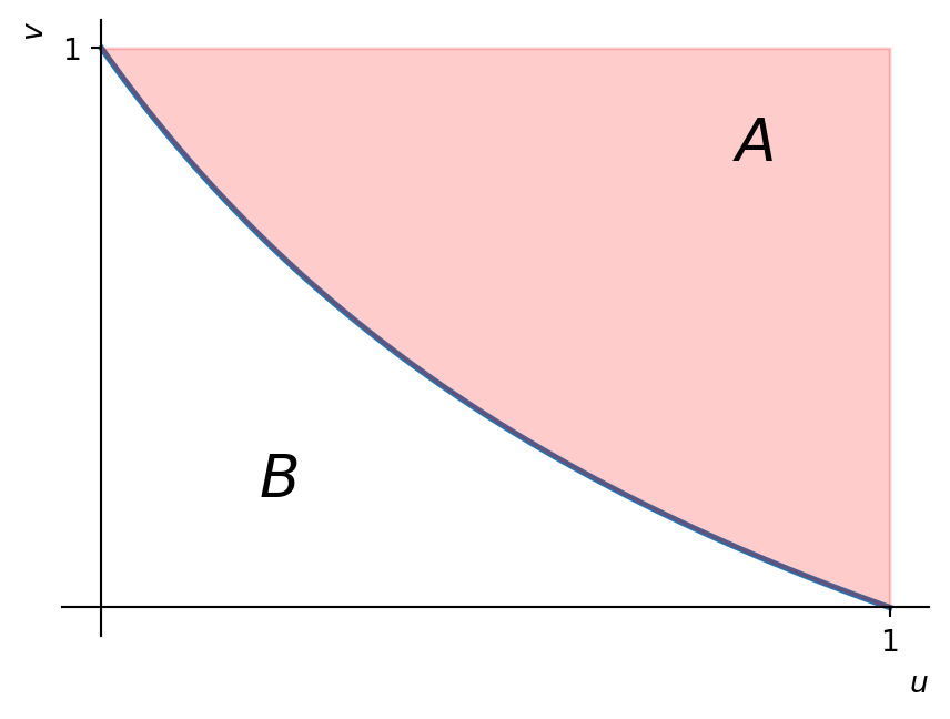
Figure 5.5: Visualising the sets $A$ and $B$, with the set $A$ in red and in blue the graph of $f$

Exercise 5.4 [**] Let’s revisit our old friend, the Clayton family of copulas from Section 4.1: \[C_\theta(u,v)=\left( \max\{u^{-\theta}+v^{-\theta}-1,0\} \right)^{-1/\theta} \quad \text{for all } u,v \in (0,1),\] where for simplicity we limit the parameter to $\theta \in (0,\infty)$.

Show that for any $\theta \in (0,\infty)$, $\lambda_L=2^{-1/\theta}$ and $\lambda_U=0$.
Recall that in Section 4.3.3, in particular in Listing 4.2, we made a sequence of scatterplots for a pair $(X,Y)$ with $\text{Unif}(0,1)$ marginals and a range of different parameter values. Have another look at those with positive parameter values. Discuss whether the values for $\lambda_L$ and $\lambda_U$ we computed in part i are consistent with what these scatterplots seem to show.

Hint (click to view)

For part i, we’ll need to use Proposition 5.3. First use the same technique as in Exercise 5.1 part iv to get rid of the “max” in the expression for $C_\theta(t,t)$, for $t$ close to $0$ and for $t$ close to $1$. You should find that in both cases we can simplify to \[C_\theta(t,t)=\left( \max\{2 t^{-\theta}-1,0\} \right)^{-1/\theta}.\] If you’re stuck with working out the limits needed in Proposition 5.3, then:

for $\lambda_L$, consider writing \[\left( 2 t^{-\theta}-1 \right)^{-1/\theta}=t \left( 2 -t^{\theta} \right)^{-1/\theta}.\]
for $\lambda_U$, consider using l’Hôpital’s rule.

For part ii, take the interpretation from Definition 5.3 and see whether you can recognise the behaviour that the values of $\lambda_L$ and $\lambda_U$ predict back in the scatterplots. Note that if $X$ and $Y$ both have a small value, then that results in a sample $(x,y)$ with small $x$ and $y$-coordinate i.e. close to the origin $(0,0)$, while if $X$ and $Y$ both have a large value, then that results in a sample $(x,y)$ with large $x$ and $y$-coordinate i.e. close to the point $(1,1)$. You should find that the values for $\lambda_L$ are quite well reflected in the scatterplots, while the value for $\lambda_U$ does not seem to be consistent with the scatterplots at all!

Full solution (click to view)

For part i, since we are given the copula, we’ll go with the expressions from Proposition 5.3. For any $t \in (0,1)$ we get that \[C_\theta(t,t)=\left( \max\{t^{-\theta}+t^{-\theta}-1,0\} \right)^{-1/\theta}=\left( \max\{2 t^{-\theta}-1,0\} \right)^{-1/\theta}.\] Much as in Exercise 5.1 part iv, for working out the limits in Proposition 5.3 we’d prefer not to have that “max” in place, so we first try to figure out which term in the maximum dominates for relevant values of $t$ so that we can simplify the “max” away.

For $\lambda_L$ we are interested in values for $t$ that are positive but close to $0$. Defining $f(t)=2 t^{-\theta}-1$ it is clear that $f(t) \to \infty$ as $t \downarrow 0$ and hence we may simplify to \[C_\theta(t,t)=\left( 2 t^{-\theta}-1 \right)^{-1/\theta}\] and hence \[\begin{align*} \lambda_L &= \lim_{t \downarrow 0} \frac{C_\theta(t,t)}{t} \\ &= \lim_{t \downarrow 0} \frac{\left( 2 t^{-\theta}-1 \right)^{-1/\theta}}{t} \\ &= \lim_{t \downarrow 0} \frac{\left( t^{-\theta} (2 -t^{\theta} \right)^{-1/\theta}}{t} \\ &= \lim_{t \downarrow 0} \frac{t \left( 2 -t^{\theta} \right)^{-1/\theta}}{t} \\ &= \lim_{t \downarrow 0} \left( 2 -t^{\theta} \right)^{-1/\theta} \\ &= 2^{-1/\theta} \end{align*} \] (of course this is one possible way of working out this limit, whatever your favourite method is!).
For $\lambda_U$ on the other hand we are interested in values for $t$ that are less than $1$ but close to it. That same function $f$ as above has the property that $f(1)=1>0$, and since it’s continuous it will be positive for all $t$ close (enough) to $1$. Therefore we again can simplify to \[C_\theta(t,t)=\left( 2 t^{-\theta}-1 \right)^{-1/\theta}\] (in fact, you could check that this is the correct expression for all $t \in (0,1)$ if you’d like!). This gives \[\begin{align*} \lambda_U &= 2-\lim_{t \downarrow 1} \frac{1-C_\theta(t,t)}{1-t} \\ &= 2-\lim_{t \downarrow 1} \frac{1-\left( 2 t^{-\theta}-1 \right)^{-1/\theta}}{t} \\ &= 2-\lim_{t \downarrow 1} \frac{-2t^{-\theta-1} \left( 2 t^{-\theta}-1 \right)^{-1/\theta-1}}{-1} \\ &= 2-\lim_{t \downarrow 1} 2t^{-\theta-1} \left( 2 t^{-\theta}-1 \right)^{-1/\theta-1} \\ &= 2-2 \cdot 1^{-\theta-1} \left( 2 \cdot 1^{-\theta}-1 \right)^{-1/\theta-1} \\ &= 0, \end{align*} \] where the third equality uses l’Hôpital’s rule and the fifth uses that because the expression we’re taking the limit of is continous in/around $t=1$ we can simply evaluate it by plugging in $t=1$.

For part ii, let’s first focus on $\lambda_L=2^{-1/\theta}$. As you can readily check, for the positive parameter values for which we have created a scatterplot in Listing 4.2, this yields the following values for $\lambda_L$ (rounded to two decimals):

$\theta$	$\lambda_L$
0.1	0.00
0.5	0.25
0.75	0.40
1	0.50
5	0.87
10	0.93
25	0.97
50	0.99
100	0.99
150	1.00

(obviously, the final value is the result of rounding up). These values seem very consistent with the behaviour we see in the scatterplots: for $\theta=0.1$ we have a very small value of $\lambda_L$, implying that small values of $X$ (so close to $0$, recall the $\text{Unif}(0,1)$ marginals) do not make small values of $Y$ more likely. Indeed in that plot, small values of $X$ come with a large variety of $Y$ values, from small to very large (i.e. close to $1$). As we increase $\theta$ and hence the value of $\lambda_L$, we indeed see that small values of $X$ are ever more accompanied by small values of $Y$ (the points with small $x$-coordinates are increasingly more concentrated near the origin, where the $y$-coordinate is small as well rather than higher up nearer the point $(0,1)$). In the plots where $\theta \geq 10$ there seems to be hardly any escape anymore to the strict rule: “if $x$-coordinate small, then also $y$-coordinate small” i.e. if $X$ small value, then $Y$ also pretty much certainly a small value. This is consistent with the values for $\lambda_L$ quite close to $1$.

Ok, that’s nice! Now we have gained some courage and confidence, let’s look at the upper tail dependence parameter. Recall that we saw that $\lambda_U=0$ for all $\theta>0$, which means that $X$ having a (very) large value does not at all make (very) large values of $Y$ more likely as well. Hmmm. But if we look at the scatterplots, it does seem an awful lot as if there is such a relationship! After all, especially for larger values of $\theta$, we see that all points with large (i.e. close to $1$) $x$-coordinates also have large $y$-coordinates. After all there are never any points near the point $(1,0)$, they’re all quite decisively near the top right corner i.e. near the point $(1,1)$! So… what is going on here, how can we explain this seeming contradiction??

The truth is that actually there is no contradiction! What we’re observing here is essentially a limitation of scatterplots combined with some very subtle behaviour of the copula. Recall that $\lambda_U=0$ gives the connection between (very) large values of $X$ and $Y$ only in the extreme limit for $t \uparrow 1$. The Clayton copula has the subtle property that it causes \[\P \big( Y > F_Y^{-1}(t) \big| X > F_X^{-1}(t) \big)\] to be quite large for $t$ until very close to $t=1$, then it suddenly drops back down to $0$. This causes a limiting value of $\lambda_U=0$, while in the scatterplot the area in which that drop happens is so close to the upper right corner point $(1,1)$ that we can’t detect it — to see it properly we would have to seriously zoom in on that upper right corner point and generate many more samples than we did to ensure enough end up in that tiny area to allow us to actually observe this effect.

So, the take home message is: scatterplots are brilliant as a quick-and-dirty tool to get a good impression of the broad characteristics of your pair of random variables/copula, but it’s regularly too blunt to properly capture quite subtle characteristics!

Exercise 5.5 [💀] This question is not very difficult, but it’s not “core” i.e. don’t worry about it for exam purposes — though it’s quite interesting I think if you haven’t seen these details before!

Let $X$ and $Y$ be two rv’s with finite (but non-zero) variance. The goal of this question is to look in a bit more detail at approximating $Y$ by a linear function of $X$ and how this relates to the correlation coefficient $\rho(X,Y)$, to underpin the claims in Section 5.2. More precisely, we would like to find $a,b \in \R$ so that $aX+b$ is as close as possible to $Y$, where we measure the distance between them using the expected squared error/distance. That is, the distance between $aX+b$ and $Y$ is given by the function $f:\R^2 \to [0,\infty)$ defined as \[f(a,b)=\E \Big[ \big( Y-(aX+b) \big)^2 \Big] \quad \text{for $a,b \in \R$.} \tag{5.27}\]

Clearly we are interested in finding values for $a$ and $b$ that minimise the function $f$ as these give the best approximation of $Y$ by $aX+b$ (at least using this metric) — i.e. in solving Equation 5.2. In parts i and ii below we use a cute technique to solve this minimisation problem that avoids using partial derivatives and (hence) avoids the problem that partial derivatives only give local extrema, not necessarily global ones.

Show that for any $a \in \R$ fixed, the function $b \mapsto f(a,b)$ has \[b_0=b_0(a):=\E[Y]-a\E[X]\] as its (unique) minimiser.

Hint: just work out the brackets in Equation 5.27 and realise that the expectations you have in your expressions are just constants as they don’t depend on $b$!
Show that the function $a \mapsto f(a,b_0(a))$ can be expressed as \[a \mapsto f(a,b_0(a)) = \var(Y)+a^2 \var(X)-2a\cov(X,Y). \tag{5.28}\] Find the minimiser of this function and deduce that the point $(\widehat{a},\widehat{b})$ given by \[\widehat{a}=\frac{\cov(X,Y)}{\var(X)}, \quad \widehat{b}=\E[Y]-\frac{\cov(X,Y)}{\var(X)} \E[X]\] is the unique global minimiser of the function $f$.

Hint: Equation 5.28 can be done in a few lines only. Keep in mind that $\var(Z)=\E[(Z-\E[Z])^2]$ as well as the standard rules for working with variances and covariances.
Deduce that we have the following relationship between the optimal choice for $a$, i.e. $\widehat{a}$, and the correlation coefficient of $X$ and $Y$: \[\rho(X,Y)=\widehat{a} \sqrt{\frac{\var(X)}{\var(Y)}}.\]

That is: the correlation coefficient can be seen as a normalised version of $\widehat{a}$, where the normalising factor equals $1$ and hence $\rho(X,Y)=\widehat{a}$ if and only if $X$ and $Y$ have equal variance. But also if this factor doesn’t equal $1$, it is always strictly positive and hence we see that the correlation coefficient is equal to $0$ resp. positive resp. negative if and only if $\widehat{a}$ is equal to $0$ resp. positive resp. negative.
Of course, nothing is ever stopping us from approximating $Y$ by $aX+b$, but that does not (at all!) mean that we are always going to end up with a very good/useful approximation! In order to check how well $\widehat{a}X+\widehat{b}$ approximates $Y$ (in the chosen distance metric), we could look at the value of $f(\widehat{a},\widehat{b})$: the smaller (i.e. closer to $0$) that guy is the smaller the distance between $\widehat{a}X+\widehat{b}$ and $Y$, and hence the happier we can be with our approximation. Now, use Equation 5.28 to show that \[f(\widehat{a},\widehat{b}) = \var(Y) \left( 1-\rho(X,Y)^2 \right).\]

After you’ve chewed through this question, have another look at Proposition 5.1 and convince yourself that that the results from parts iii and iv above indeed give rise to the claims made in that proposition!

Hint (click to view)

For part i, working out the brackets you should find that $b \mapsto f(a,b)$ rewrites to \[b \mapsto \E[Y^2]-2a\E[XY]-2b\E[Y]+a^2 \E[X^2]+2ab \E[X]+b^2,\] and then it’s a routine matter of differentation e.g.

For part ii, just pick up the worked out expression for $f(a,b)$ from part i, and plug the expression for $b_0$ from part i in there. Also don’t forget the rules $\cov(Y,-aX)=-a\cov(Y,X)$ and $\cov(Y,X)=\cov(X,Y)$, which follow immediately from its def (cf. Definition 5.1).

For parts iii & iv, a little bit of algebra should do the trick for each of these.

Full solution (click to view)

For part i, fixing some $a \in \R$, working out the brackets and using the linearity property of expectations we can write \[\begin{align*} b \mapsto f(a,b) &= \E \left[ \left( Y-(aX+b) \right)^2 \right] \\ &= \E \left[ \big( Y-(aX+b) \big) \big( Y-(aX+b) \big) \right] \\ &= \E[Y^2]-2a\E[XY]-2b\E[Y]+a^2 \E[X^2]+2ab \E[X]+b^2. \end{align*} \] Keeping in mind that $a$ is a fixed constant, as are all the expectations appearing there, to find the minimiser of this function is simply a matter of either recognising that it is a second order polynomial and employing the standard expression for its minimiser, or to differentiate it.

For part ii, writing $b_0(a)=\E[Y-aX]$ and plugging this in: \[\begin{align*} a \mapsto f(a,b_0(a)) &= \E \left[ \big( Y-aX - \E[Y-aX] \big)^2 \right] \\ &= \var(Y-aX) \notag \\ &= \var(Y)+\var(-aX)+2\cov(Y,-aX) \notag \\ &= \var(Y)+a^2\var(X)-2a\cov(X,Y) \end{align*} \tag{5.29}\] where we used the standard rules for working with variances plus the rules $\cov(Y,-aX)=-a\cov(Y,X)$ and $\cov(Y,X)=\cov(X,Y)$ which both follow immediately from its def (cf. Definition 5.1). Now it is again a straightforward computation of its derivative and/or recognising this expression as a second order polynomial.

We can now conclude that the point $(\widehat{a},\widehat{b})$, where $\widehat{b}:=b_0(\widehat{a})$ (cf. part i), is indeed the global minimiser of the function $f$. After all, for any point $(a_1,b_1)$ we have that \[f(a_1,b_1) \geq f(a_1,b_0(a_1)) \geq f(\widehat{a},b_0(\widehat{a})),\] the first inequality by part i and the second inequality by the work we have done in this part.

For part iii, this is pretty straightforward from the definition of $\rho$ (cf. Definition 5.1) with a little bit of algebra: \[\begin{align*} \rho(X,Y) &= \frac{\cov(X,Y)}{\sqrt{\var(X)\var(Y)}} \\ &= \frac{\cov(X,Y)}{\var(X)} \frac{\var(X)}{\sqrt{\var(X)\var(Y)}} \\ &= \widehat{a} \frac{\var(X)}{\sqrt{\var(X)\var(Y)}} \\ &= \widehat{a} \frac{\sqrt{\var(X)} \sqrt{\var(X)}}{\sqrt{\var(X)}\sqrt{\var(Y)}} \\ &= \widehat{a} \sqrt{\frac{\var(X)}{\var(Y)}}. \end{align*} \]

For part iv, plugging the expression for $\widehat{a}$ in Equation 5.29 and again using Definition 5.1 we see that we can indeed write \[\begin{align*} f(\widehat{a},\widehat{b}) &= \var(Y)+\frac{\cov(X,Y)^2}{\var(X)} -2 \frac{\cov(X,Y)^2}{\var(X)} \\ &= \var(Y) -\frac{\cov(X,Y)^2}{\var(X)} \\ &= \var(Y) \left( 1-\frac{\cov(X,Y)^2}{\var(X)\var(Y)} \right) \\ &= \var(Y) \left( 1-\rho(X,Y)^2 \right). \end{align*} \]